NICE DSU TECHNICAL SUPPORT DOCUMENT 15: COST-EFFECTIVENESS MODELLING USING PATIENT-LEVEL SIMULATION

1

NICE

DSU

TECHNICAL

SUPPORT

DOCUMENT

15:

COST-EFFECTIVENESS

MODELLING

USING

PATIENT-LEVEL

SIMULATION

R

D

S

U

Sarah Davis, Matt Stevenson, Paul Tappenden, Allan Wailoo

School of Health and Related Research, University of Sheffield

Decision Support Unit, ScHARR, University of Sheffield, Regent Court, 30 Regent Street Sheffield, S1 4DA

Tel (+44) (0)114 222 0734

E-mail [email protected] Website www.nicedsu.org.uk Twitter @NICE_DSU

2

A

D

S

U

The Decision Support Unit (DSU) is a collaboration between the Universities of Sheffield, York and Leicester. We also have members at the University of Bristol, London School of Hygiene and Tropical Medicine and Brunel University. The DSU is commissioned by The National Institute for Health and Care Excellence (NICE) to provide a research and training resource to support the Institute's Technology Appraisal Programme. Please see our website for further information www.nicedsu.org.uk

A

T

S

D

The NICE Guide to the Methods of Technology Appraisal is a regularly updated document that provides an overview of the key principles and methods of health technology assessment and appraisal for use in NICE appraisals.1 The Methods Guide does not provide detailed advice on how to implement and apply the methods it describes. This DSU series of Technical Support Documents (TSDs) is intended to complement the Methods Guide by providing detailed information on how to implement specific methods.

The TSDs provide a review of the current state of the art in each topic area, and make clear recommendations on the implementation of methods and reporting standards where it is appropriate to do so. They aim to provide assistance to all those involved in submitting or critiquing evidence as part of NICE Technology Appraisals, whether manufacturers, assessment groups or any other stakeholder type.

We recognise that there are areas of uncertainty, controversy and rapid development. It is our intention that such areas are indicated in the TSDs. All TSDs are extensively peer reviewed prior to publication (the names of peer reviewers appear in the acknowledgements for each document). Nevertheless, the responsibility for each TSD lies with the authors and we welcome any constructive feedback on the content or suggestions for further guides.

Please be aware that whilst the DSU is funded by NICE, these documents do not constitute formal NICE guidance or policy.

Professor Allan Wailoo

3

Acknowledgements

The authors wish to acknowledge the contributions of Jaime Caro, Mike Pidd, Steve Chick and the team at NICE, led by Gabriel Rogers, who provided peer review comments on the draft document. They also wish to acknowledge Gabriel Rogers for developing the object-orientated version of the Visual Basic model. In addition they would like to acknowledge Paul Edwards and the team from TreeAge who collaborated on developing the example TreeAge models, provided material for the TSD on implementation of patient-level simulation within TreeAge and provided general comments on the draft. They would also like to acknowledge Jon Minton who developed the R code and Paul Richards who assisted with its validation and Jenny Dunn who assisted with formatting the document.

The production of this document was funded by the National Institute for Health and Care Excellence (NICE) through its Decision Support Unit. The views, and any errors or omissions, expressed in this document are of the authors only. NICE may take account of part or all of this document if it considers it appropriate, but it is not bound to do so.

This report should be referenced as follows:

Davis, S., Stevenson, M., Tappenden, P., Wailoo, A.J. NICE DSU Technical Support Document 15: Cost-effectiveness modelling using patient-level simulation. 2014. Available from http://www.nicedsu.org.uk

4

C

1.  INTRODUCTION... 7 

2.  A TAXONOMY OF MODELLING APPROACHES ... 8 

2.1.  DEFINING PATIENT-LEVEL AND COHORT MODELLING APPROACHES ... 8 

2.2.  DEFINITION OF STOCHASTIC AND ANALYTIC EVALUATION ... 9 

2.3.  DECISION TREE ANALYSIS ... 10 

2.4.  STATE-TRANSITION MODELS ... 11 

2.5.  DISCRETE EVENT SIMULATION ... 11 

2.6.  HANDLING OF TIME WITHIN THE MODEL ... 13 

3.  IDENTIFYING WHEN A PATIENT-LEVEL SIMULATION MAY BE PREFERABLE TO A COHORT APPROACH ... 14 

3.1.  MODEL NON-LINEARITY WITH RESPECT TO HETEROGENEOUS PATIENT CHARACTERISTICS ... 14 

3.2.  PATIENT FLOW DETERMINED BY TIME SINCE LAST EVENT OR HISTORY OF PREVIOUS EVENTS ... 15 

3.3.  AVOIDING LIMITATIONS ASSOCIATED WITH USING A DISCRETE TIME INTERVAL ... 17 

3.4.  DEVELOPING A FLEXIBLE MODEL AS AN INVESTMENT FOR FUTURE ANALYSES ... 18 

3.5.  MODELLING SYSTEMS WHERE PEOPLE INTERACT WITH RESOURCES OR OTHER PEOPLE .. ... 18 

3.6.  NEED FOR PROBABILISTIC SENSITIVITY ANALYSIS TO ASSESS DECISION UNCERTAINTY .. ... 19 

4.  IMPLEMENTING A SIMPLE MODEL WHICH INCORPORATES PATIENT HISTORY USING DIFFERENT APPROACHES ... 20 

4.1.  GENERAL DISCRETE EVENT FRAMEWORK ... 21 

4.2.  IMPLEMENTING A DES IN A GENERIC PROGRAMMING LANGUAGE ... 25 

4.2.1.  Visual Basic DES ... 25 

4.2.2.  DES in R ... 27 

4.3.  IMPLEMENTING A DES IN TREEAGE PRO ... 28 

4.4.  DES IN A BESPOKE SIMULATION PACKAGE (SIMUL8) ... 31 

4.5.  TECHNIQUES REQUIRED TO IMPLEMENT A DES ... 34 

4.5.1.  Sampling from a distribution ... 34 

4.5.2.  Sampling time to death from national life-table data ... 35 

4.5.3.  Calculating discount rates for costs and QALYs accrued over an extended time period ... 36 

4.5.4.  Estimating acceleration factors from hazard ratios when time to event data follow a Weibull distribution ... 37 

4.6.  PATIENT-LEVEL STATE-TRANSITION FRAMEWORK ... 38 

4.6.1.  Practical difficulties of implementing a patient-level state-transition model within a spreadsheet package. ... 43 

5

4.6.2.  Implementing a patient-level state-transition model in TreeAge Pro ... 44 

5.  GOOD MODELLING PRACTICE FOR PATIENT-LEVEL SIMULATIONS ... 47 

5.1.  STRUCTURING A PATIENT-LEVEL SIMULATION ... 47 

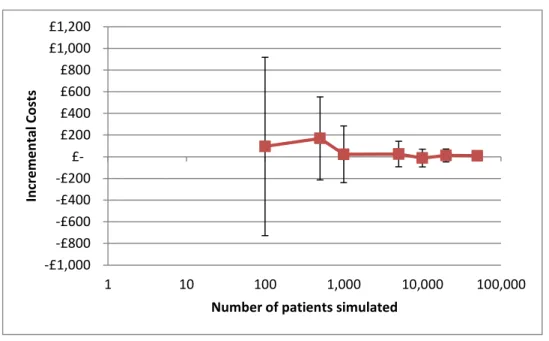
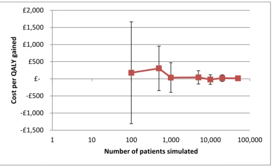
5.2.  ESTABLISHING THE NUMBER OF INDIVIDUAL PATIENTS TO SIMULATE ... 48 

5.3.  CONDUCTING PROBABILISTIC SENSITIVITY ANALYSIS ... 51 

5.4.  THE RELATIVE IMPORTANCE OF FIRST- AND SECOND- ORDER UNCERTAINTY ... 53 

5.5.  TRANSPARENT REPORTING OF PATIENT-LEVEL SIMULATIONS ... 53 

5.6.  VALIDATING PATIENT-LEVEL SIMULATIONS ... 54 

6.  REFERENCES ... 59 

Tables and figures

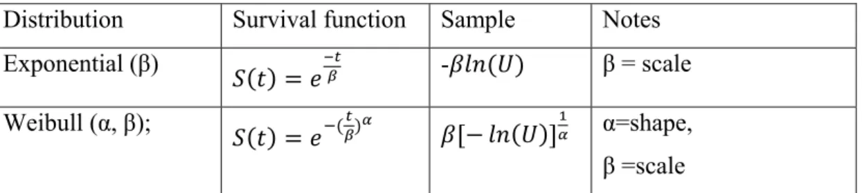
Table 2: Avoiding / identifying errors in patient-level simulations ... 57 

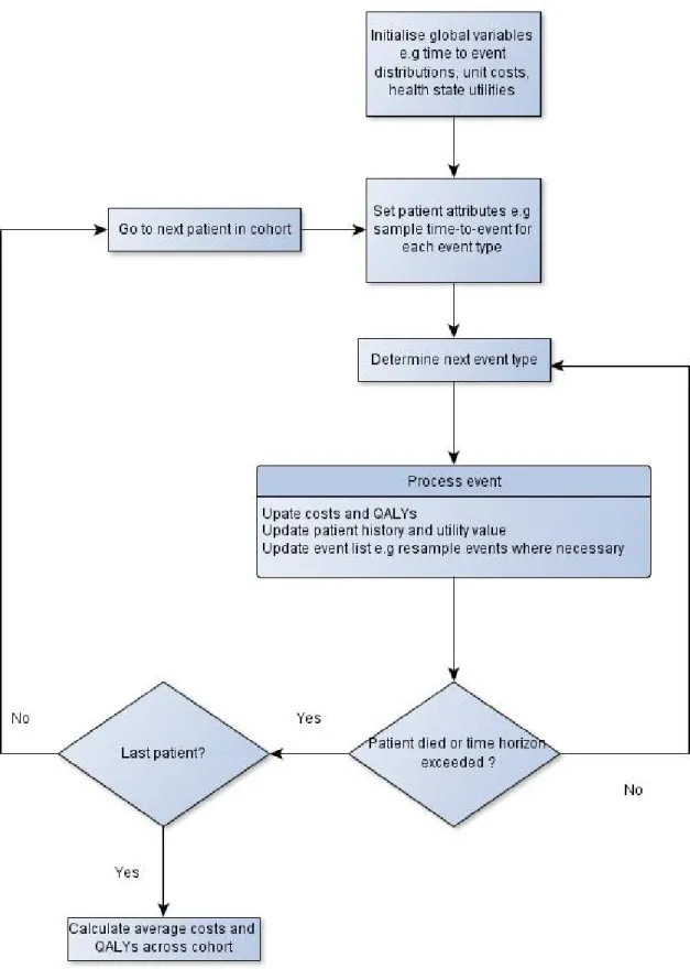
Figure 1: Key model logic for a DES (when simulating one patient at a time) ... 24 

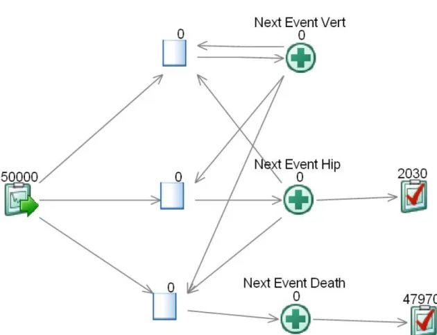
Figure 2: Structure for DES implemented in TreeAge Pro ... 30 

Figure 3: Graphical representation of example model in SIMUL8 ... 33 

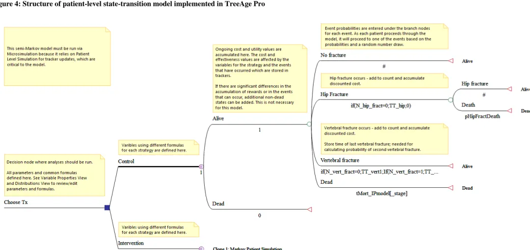
Figure 4: Structure of patient-level state-transition model implemented in TreeAge Pro ... 46 

Figure 5: A plot of incremental costs in relation to the number of patients simulated. ... 49 

Figure 6: A plot of incremental QALYs gained in relation to the number of patients simulated. ... 49 

6

A

bbreviations

ATF Accelerated time failure

CHEERS Consolidated Health Economic Evaluation Reporting Standards

CI Confidence interval

DES Discrete event simulation

DSU Decision Support Unit

HTA Health Technology Assessment

ICER Incremental cost-effectiveness ratio

ISPOR-SMDM International Society for Pharmacoeconomics and Outcomes Research - Society for Medical Decision Making

NICE National Institute for Health and Care Excellence OR-MS Operational Research – Management Science pEVPI Partial expected value of perfect information

PSA Probabilistic Sensitivity Analysis

TA Technology Appraisal

TSD Technical Support Document

7

1.

INTRODUCTION

Economic models which estimate the relative costs and benefits of alternative technologies are an essential element of the National Institute for Health and Care Excellence’s (NICE’s) Technology Appraisal (TA) process. Such models are designed to estimate the mean costs and benefits of alternative health technologies for the population likely to be affected by a particular decision. In some cases a single decision is made for the whole population falling within the scope of the TA, whilst in other cases, where the costs and benefits are expected to differ within the population, different decisions are made for different subgroups of the population specified in the scope. However, in both cases the TA Committee’s guidance is based on the average costs and benefits across some specified population rather than the individual outcomes occurring at the patient level.

Economic models can use either a patient-level or cohort-level modelling approach to estimate the expected costs and outcomes across a particular population. In a patient-level simulation, the outcomes are modelled for individual patients and then the average is taken across a sufficiently large sample of patients, whilst in a cohort-level model the outcomes are estimated for the cohort as a whole without considering the outcomes for individual patients within that cohort. The optimal approach will depend on the particular nature of the decision problem being modelled and therefore needs to be assessed on a case-by-case basis.2 It is important that the choice between using a patient-level simulation and a cohort-level modelling approach is given careful consideration and is properly justified in the model description, as the models used to inform NICE TAs have sometimes been criticised on this basis.3

The decisions of NICE Technology Appraisal Committees are dependent on both the mean expected costs and benefits and the uncertainty in those means, arising from uncertainty in the evidence used to inform the economic model. Therefore it is important that decision uncertainty is correctly estimated regardless of the choice of model structure.4 The standard way to assess the decision uncertainty associated with the model parameters is through probabilistic sensitivity analysis (PSA), in which samples are taken from distributions reflecting the uncertainty in the model parameters and this uncertainty is propagated through the model. In the past this has been viewed as a barrier to the use of patient-level simulation due to the computational requirements of simulating both a large number of patients to obtain

8

a precise estimate of the expected costs and benefits, and a large number of parameter samples to evaluate the uncertainty surrounding the expected costs and benefits.5 However, we describe here how patient-level simulation can be combined with PSA to meet the information needs of NICE TA Committees.

The aims of this Technical Support Document (TSD) on patient-level simulation are to:

 Increase awareness of patient-level modelling approaches and highlight the key differences between patient-level and cohort-level modelling approaches.

 Provide guidance on situations in which patient-level modelling approaches may be preferable to cohort-level modelling approaches.

 Provide a description of how to implement a patient-level simulation illustrated with example models.

 Provide guidance on good practice when developing and reporting a patient-level simulation to inform a NICE TA.

The example models are built in the standard software packages (Microsoft Excel®, TreeAge Pro®, R6) accepted by NICE without prior agreement.7,8 We have also provided one example of a discrete event simulation implemented in a bespoke simulation package (SIMUL8®). It should be noted that permission from NICE must be sought in advance to submit a model implemented in a non-standard software package such as a bespoke simulation package.

The focus of this document is on the use of economic models to inform NICE TAs. Systems incorporating interactions between patients are not a common feature within TA and therefore this document focuses on the application of patient-level simulation to systems where patients can be assumed to be independent. However, a brief discussion of the application of patient-level simulation to situations involving patient interaction is given in section 3.5.

2.

A TAXONOMY OF MODELLING APPROACHES

2.1.

D

-

Economic models estimate the costs and benefits across the target population by considering the outcomes for a group of patients which represent the target population. Here we define a

9

patient-level simulation as any model which estimates the mean costs and benefits for that group of patients by considering the costs and benefits of each individual within the group. (These types of models have sometimes been referred to as ‘individual sampling models’).9,10 Conversely a cohort model is any model which estimates the outcomes for the group of patients without explicitly considering the outcomes of each individual patient. A cohort model may allow for some variability in patient outcome according to patient characteristics defined at the start of the model, but it is not a patient-level simulation unless the outcomes are evaluated at the patient-level. For example, a cohort model may evaluate outcomes for a group of patients in which 40% of the starting cohort is female and may apply different mortality rates for males and females, or it may allow different treatment pathways for subgroups who are unable to tolerate a particular second-line treatment. In both cases this would require certain subgroups of the cohort to be tracked separately through the model. Therefore, a cohort modelling approach does not imply that there is no variation in patient characteristics or outcomes within the cohort, although any variation in outcomes is likely to be captured for broad categories of patients rather than at an individual level.

2.2.

D

Models that can be evaluated without the need to randomly sample from parameter distributions are said to be evaluated analytically. Stochastic evaluation refers to the process of allowing certain values within the model to vary randomly according to a specified distribution and taking the mean model outcome over a large number of model runs. Stochastic evaluation allows the distribution of outcomes to be estimated in addition to their mean value, which may also be of interest to decision makers. Different types of stochastic variation can be incorporated within a decision analytic model.

In models which consider individual-level patient heterogeneity, stochastic variation can be incorporated at the level of patient characteristics. In such models, the mean model outcomes are estimated across a group of patients whose starting characteristics are sampled from distributions.

Stochastic variation may also occur at the decision node, state-transition or time-to-event level allowing random variation in the model trajectory for an individual patient, in a manner

10

which does not necessarily depend on the patient’s characteristics at the start of the model. This type of stochastic variation is referred to here as stochastic uncertainty.

Finally, stochastic variation can occur at the parameter level, where parameter values are sampled from a distribution reflecting the uncertainty in their population mean value and this uncertainty is propagated through the model to determine the resulting uncertainty in the expected model outcomes. This type of stochastic evaluation of parameter uncertainty is generally referred to in this context as probabilistic sensitivity analysis (PSA).11 PSA is a requirement of models submitted to the NICE Technology Appraisal Programme.1

Care should be taken when discussing the appropriate modelling approach to distinguish between the different types of stochastic evaluation that can be incorporated within the model to avoid confusion between patient heterogeneity, stochastic uncertainty and parameter uncertainty.12 For example, it is important not to include parameters which reflect patient heterogeneity within the PSA. Koerkamp et al. provide a clear description of the different

types of stochastic variation that can be incorporated and combined within a health economic evaluation and how these can be evaluated to provide different information on the uncertainty and variability associated with expected model outcomes.12

2.3.

D

Decision tree analysis estimates the likelihood of various outcomes occurring using a probability tree and then applies associated pay-offs, the costs and benefits in this context, for each branch of the tree. Decision tree analysis does not explicitly model the timing of outcomes, making it necessary for the analyst to adjust pay-offs for events occurring in the future to allow for discounting. In the past, decision tree analysis was commonly employed to model a cohort of homogeneous patients analytically using mean parameter values.5 However, NICE’s requirement for PSA has resulted in probabilistic evaluation of parameter uncertainty becoming common place. It should however be noted that decision trees can also be evaluated stochastically allowing each individual to follow a unique path through the decision tree based on samples drawn from statistical distributions, as opposed to estimating the proportion following each path in the traditional manner.10 Therefore, a decision tree framework can be compatible with a patient-level simulation approach.

11

2.4.

S

-

State-transition models consist of a discrete set of mutually exclusive health states which are evaluated at regular intervals to determine the population of each health state. The flow of patients through the model over time is determined by the application of a transition matrix which defines the probability of moving between each state within one cycle. State-transition models are often synonymously referred to within a health economic context as ‘Markov models’, although strictly the use of the term ‘Markov’ should be limited to models which display the ‘Markovian property’ in which transitions are dependent only on the state in which the patient resides and not on anything that occurred before they arrived in that state or the duration of time they have occupied that state. This is sometimes referred to as a ‘memoryless’ process. The simplest form of a state-transition model is one in which a fixed transition matrix is applied every cycle giving a time homegenous Markov chain, although this approach can also be extended to give a Markov process in which time varying transition matrices are allowed. The term ‘Markov model’ has often been used synonymously with the term ‘cohort model’ within the health economic context because Markov state-transition models are so often employed to model cohorts of patients. Cohort state-transition models evaluate the proportion of patients within the cohort who reside within each of the model states for each model cycle. They are also widely combined with PSA to provide an estimate of the distribution of costs and benefits expected for a cohort of homogeneous patients with average characteristics. However, as with decision trees, they can also be evaluated stochastically using samples drawn from statistical distributions to determine whether an individual patient experiences a particular transition given the probability of that transition occurring in that particularly cycle.13 Therefore, a state-transition model framework is also compatible with a patient-level simulation approach.

Guidance on developing state-transition models has been produced by the ISPOR-SMDM Modeling Good Research Practices Task Force.14

2.5.

D

A discrete event simulation (DES) is concerned with the events that occur during the lifetime of individual entities. As the individual entities are usually patients in this context, DESs are inherently patient-level and the expected outcome for the population of interest can only be

12

reliably estimated by simulating a sufficiently large number of patients. The simulation maintains a list of the time to each possible event, as sampled for each individual patient, and the simulation clock is advanced from one event to the next. Therefore, unless events are scheduled to happen at regular intervals, the simulation clock will step forward at irregular intervals which are dependent on the sampled times between subsequent events. The simulation tracks patient attributes (both continuous and categorical) and global variables such as total costs and quality adjusted life-years (QALYs). These are updated each time an event occurs. Individual entities can experience an event of the same type more than once if after the first event is processed another event of the same type is scheduled. The time to future events can be made dependent on patient attributes including their history of previous events. Continuous patient attributes can be updated at specified time intervals by setting up events which occur at regular intervals such as annual increases in age.

It is also possible within a DES framework to allow patients to interact with other patients or with other entities which are defined as resources within the simulation such as doctors, appointment slots, equipment etc. These resources may be constrained leading to the formation of queues where the next event can only be processed when a particular resource is available. Such flexibility allows for very complex systems to be modelled incorporating factors such as infection and service capacity, although these are often not necessary within a TA context.15 (See section 3.5 for a brief discussion of model structures which are suitable for modelling systems with interaction between individuals or constrained resources.)

Discrete event simulations are inherently patient-level and must be evaluated stochastically to produce precise estimates of the expected costs and benefits across a specific patient population. This is the key trade-off against the increased level of flexibility they provide. The main model inputs driving flow through the model are the distributions of time-to-event for each event type. In DES these time-to-event values are sampled for individual patients from probability distributions.

One of the benefits of using a DES approach is that it may have more face validity with clinicians and patients who may appreciate the transparency of being able to visualise (or, with some software packages, see animations of) individual patients experiencing disease outcomes and accruing costs and health benefits. Although care should be taken that this

13

additional realism does not result in more trust being placed in the model than is warranted and that the desire for face validity does not result in models that are unnecessarily complex.

Guidance on developing DES has been produced by the ISPOR-SMDM Modeling Good Research Practices Task Force.16

2.6.

H

Decision tree analysis estimates the likelihood of various outcomes occurring and the associated pay-offs without explicitly modelling the timing of outcomes. It is therefore generally used to model events occurring over a short time-horizon or where the exact timing of the event is unimportant. State-transition models employ a discrete time approach to estimate the number of patients experiencing particular health states at fixed time-points which are determined by the cycle length and the time horizon. Given that real-life clinical events can occur at any point in time, the discrete time approach employed within a state-transition model essentially provides a numerical approximation to the real-life scenario. The accuracy of the approximation can be increased by incorporating continuity corrections such as a half-cycle correction and by reducing the cycle length.17 Reducing the cycle length until there is no appreciable effect on the model outcomes is recommended.17 This may be achieved at longer cycle lengths if a continuity correction is applied.17 Discrete event simulations progress through the times at which specific events happen for particular individual entities, based on samples from discrete or continuous distributions, allowing events to occur at any time point. However a DES cannot be considered to be a true continuous time model as it simulates events according to intervals in which the state of the system is known to have changed.18

14

3.

IDENTIFYING WHEN A PATIENT-LEVEL SIMULATION MAY BE

PREFERABLE TO A COHORT APPROACH

3.1.

M

-

CHARACTERISTICS

If there are factors which vary between patients (e.g. age) which have a non-linear relationship with the model outcomes (e.g. costs and QALYs), then estimating the model outcomes for a cohort of patients using only average characteristics (e.g. mean age at starting treatment) will provide a biased estimate of the average outcome across the population to be treated.

Where such factors can be identified in advance of starting treatment, it may be possible to conduct subgroup analysis to determine the average outcome in subgroups of patients defined using broad categories of the factor of interest (e.g. 5 year age bands), provided the outcomes within those subgroups are expected to be reasonably homogeneous. This would allow either for separate recommendations to be made for each subgroup, or for a weighted average to be taken across the subgroups to make a single recommendation across the whole population. The latter may be necessary in situations where legal or ethical considerations would make separate recommendations unacceptable.

In some cases it is known that a certain factor affects outcomes, but it cannot be determined which patients will be affected prior to treatment initiation, making separate recommendations impossible. Griffin et al. give disease progression rate, within the context

of a cancer screening program, as an example of one such variable.5 It may not be possible to know which patients are likely to experience faster disease progression prior to offering screening, but if disease progression has a non-linear relationship with outcomes, it would be necessary to include the variability in disease progression within the model to obtain an unbiased estimate of the mean outcomes across the cohort offered screening. In these situations an approximate solution may sometimes be obtained by averaging across analytically evaluated models, in a manner similar to the averaging of outcomes across subgroups described above.

15

The use of subgroup analysis and model averaging to address patient heterogeneity becomes problematic when the number of categories required to define groups with homogeneous outcomes becomes large, either due to the presence of continuous variables requiring granular categorisation or due to the presence of many interacting factors. In such cases, a patient-level simulation may be preferable, as a group of patients can be simulated with characteristics sampled from the relevant population distributions. The expected costs and benefits across the sampled group should then provide an unbiased estimate provided that a sufficiently large sample is simulated and any covariance between the different patient characteristics is correctly taken into account.

When deciding on an appropriate modelling approach, consideration should be given to the likely relationship between characteristics which may vary within the population and the model outcomes. In some cases it may be possible to see before building the model that such a non-linear relationship exists by considering the proposed model structure and the functional form of any relationships that are to be included within the model. In other cases it may be necessary to build the model and test it for linearity with respect to patient characteristics. Where the relationship between patient characteristics and model outcomes is found to be, or could reasonably be expected to be non-linear, a patient-level simulation which incorporates patient heterogeneity should be conducted to obtain an unbiased estimate of the mean outcomes unless this can be avoided through appropriate subgroup analysis.

3.2.

P

PREVIOUS EVENTS

As described earlier, state-transition models often employ a Markovian assumption in which it is assumed that future events are independent of past events. This makes it difficult to model situations where the likelihood of future state transitions is dependent on the time since a previous transition (e.g. time on current treatment) or the history of previous events (e.g. previous fracture increases risk of further fractures). Additional states are sometimes added to state-transition models in order to allow the patients’ progress through the model to be dependent on their history as well as their current health state. The history of previous events may be incorporated by replicating states so that patients who have a particular history are handled within a separate replicate state. The dependence on time since the last transition may be incorporated by using a series of replicate states allowing the patient to move to a

16

different state each cycle to record the passage of time even though there is no change in their actual health state. These are sometimes referred to as ‘tunnel states’. Ultimately there is a limit on how many such replicate states can be incorporated before the cohort Markov state-transition approach becomes unwieldy.

One solution is to keep the state-transition framework but to evaluate the model using a patient-level simulation in which a single patient moves between health states stochastically. As only one patient is evaluated at any one time, fewer health states need to be defined as a time /history dependent transition matrix can be employed where the transition matrix for later cycles is dependent on the occupation of health states by that individual patient at earlier time points. In this case the need for a stochastic evaluation is being traded against a reduction in the number of unique health states that are required to be enumerated explicitly as part of the model. It should be noted that, depending on the complexity of the clinical scenario being modelled, the number of logical rules required to make the transition matrices dependent on the patient’s previous history, or the occupation time within each state, may make programming errors difficult to detect if the model is implemented within a spreadsheet package. When implemented in TreeAge (“Microsimulation mode”), tracker variables can be used to capture prior events of significance and to drive the transition matrix in a more transparent manner.

One innovative approach that allows factors such as time or patient history to be incorporated in a cohort state-transition model is to define the transition matrix as a multi-dimensional array. This allows a cohort model to be implemented where the transition probability is dependent on more factors than just the start and finishing state giving a non-Markov cohort state-transition model. The additional dimensions may be time since a particular event, patient characteristics or the patient’s history of previous events. Hawkins et al. used this

approach when modelling epilepsy treatments, where the probability of treatment failure declines over time.19 In their model a unique probability was defined for each possible transition, for each model cycle, giving a 3 dimensional transition matrix (dimensions are starting state, finishing state and time cycle). This method requires the use of software which can support multi-dimensional arrays, and in this case the model was implemented in the statistical programming language R.6 This approach eliminates the need for stochastic evaluation, and could in theory be applied in more complex situations where other dimensions are used to incorporate patient history or characteristics. However, populating

17

and validating such a complex transition matrix may prove more difficult that implementing a stochastic patient-level simulation.

An individual patient-level methodology is likely to provide a more efficient and parsimonious solution than trying to implement a cohort model in situations where there is substantial non-Markovian behavior due to its ability to track individual patients and record their event history and use this to update their risk of future events. A further advantage of the DES framework is that where the risk of certain events occurring changes over time, this can be handled by sampling a single time to event estimate from a non-exponential time-to-event distribution which is easier and more efficient than calculating time-dependent transition probabilities for each cycle in a patient-level state-transition model.

3.3.

A

INTERVAL

As described earlier, a state-transition model is essentially a discrete time approximation to a continuous real-life process. The application of this approximation may introduce bias if not implemented correctly. For example, the transition matrix needs to reflect the fact that multiple transitions may occur within a single cycle giving a non-zero probability for some transitions which cannot occur as a direct transition. Soares et al. describe how bias can be

introduced by incorrectly discretising a continuous flow process.17 This bias is reduced if the cycle length is shortened to a value where multiple transitions within one cycle are extremely unlikely and therefore theoretically the bias could be avoided simply by selecting a small enough cycle length. However, as pointed out by Caro, some diseases combine periods of rapid events with long periods where no events occur.20 In such cases the need for very short time cycles to accurately capture rapidly occurring events may make the model large and slow to evaluate over the required time frame. As the simulation clock within a DES steps forward in time from one event to the next, it may prove to be a more efficient modelling framework in situations such as these where multiple events can occur in quick succession followed by periods of inactivity.

18

3.4.

D

ANALYSES

Discrete event simulations are particularly flexible models which can be easily adapted to incorporate additional events or patient attributes and as such may lend themselves to iterative decision making processes or repeated use. Adapting decision tree or state-transition models to include additional health states or patient attributes can be time consuming, particularly if the model is implemented within a spreadsheet package, and this may limit the ability of the decision analysts to respond to criticisms raised during the TA process.

If a whole disease model is required which may be used across a range of different decision problems such as prevention, treatment and screening decisions, then it may be easier to develop that whole disease model using a patient-level simulation approach,21 _{and in} particular a DES framework, as these types of models are generally easier to adapt. Such an investment in a whole disease model may not seem worthwhile in the context of a single technology appraisal, where the economic model is developed by the manufacturer or sponsor of the technology to inform guidance on a single technology with a single indication. However, it may be justifiable for multiple technology appraisals, where Technology Assessment Groups develop models to assess the cost-effectiveness of more than one technology for one or more indications and these models are sometimes updated and re-used across several different TAs. In this context, the development of flexible whole disease models which can be easily adapted to inform several different decisions would increase decision making consistency across NICE’s work programme by allowing a consistent set of model assumptions to be applied within a particular disease area. (A similar argument could be made for the development of flexible whole disease models within NICE’s Clinical Guideline Programme).

3.5.

M

OTHER PEOPLE

Patient-level simulations may be particularly useful when modelling situations where people interact with other people or compete for resources that are constrained in some way such as healthcare staff, appointment slots or equipment. Systems incorporating patient interaction are not a common feature within Technology Appraisals, but are mentioned here for

19

completeness. State-transition models built using TreeAge can be run as patient-level simulations in parallel to capture interactions between patients or with system resources. However other modelling approaches may be better suited to problems where these are significant components. A DES is an obvious choice of modelling framework in such situations although there are some alternative model structures. The ISPOR-SMDM Modelling Good Research Practices Taskforce highlight dynamic transmission, DES and agent-based models as being applicable in situations where there are interactions between individuals, which may be due to disease transmission or due to the allocation of constrained resources.2 Both DES and agent-based approaches model at the patient-level whereas many dynamic transmission models employ a cohort-level system dynamics approach.2,22 Readers are referred to Brennan et al.’s paper on model taxonomy which includes a list of questions

that can be used to select an appropriate model.10

3.6.

N

UNCERTAINTY

The need for PSA has in the past been cited as a reason for choosing a model structure which allows analytic rather than stochastic evaluation of the model outcomes.5 When evaluating the decision uncertainty in a patient-level simulation using PSA it is usually necessary to run two nested simulation loops. The inner loop evaluates the outcomes across the simulated population for the given parameter values, and the outer loop samples those parameter values to reflect uncertainty in the model inputs. In a cohort-level model, only the outer loop is required, thus PSA computation time for a cohort-level model is likely to be lower than for an equivalent patient-level model. However with modern PC specifications this additional computation time may not be overly restrictive. Furthermore, the computation time for the inner loop may be reduced by keeping the patient-level simulation as efficient as possible. A DES, where calculations occur only at the times when events occur is likely to be much more efficient to evaluate stochastically than a patient-level state-transition model where calculations are needed every cycle for every simulated patient.

Further advice on conducting PSA and the relative importance of first and second order uncertainty within patient-level models can be found in section 5.3 and 5.4.

20

4.

IMPLEMENTING A SIMPLE MODEL WHICH INCORPORATES

PATIENT HISTORY USING DIFFERENT APPROACHES

Here we introduce a simple model for assessing the cost-effectiveness of osteoporosis treatments in order to demonstrate how such a model could be represented using a variety of modelling frameworks. This model is not a comprehensive model for assessing osteoporosis treatments, but it is intended only as a teaching example. The key model assumptions are:

 Patients start with a history of no previous fractures and a baseline utility of 0.7

 The only types of fractures that can occur are hip fractures and vertebral fractures

 Patients can experience up to one hip fracture

 Patients can experience up to two vertebral fractures

 Fractures result in one-off costs which are incurred at the time of the fracture (£7000 for hip and £3000 for vertebral)

 Fractures result in a life-long utility multiplier being applied to the patient’s pre-fracture utility (0.75 for hip pre-fracture, 0.90 for first vertebral pre-fracture, 1 for second vertebral fractures). So for example, a patient who has had a hip fracture and two vertebral fractures will have a utility of 0.7x0.75x0.9x1 =0.4725

 Patients in the control arm incur no costs other than those associated with fractures

 Patients in the intervention arm incur a fixed cost per day for treatment from the start of the model until death (equivalent to £500 p.a.)

 Time (in years) to hip fracture is described as a Weibull distribution with shape of 4 and scale of 10.

 Time (in years) to vertebral fracture is described as a Weibull distribution with shape 2 and scale of 8.

 Intervention doubles the expected time to hip fracture and expected time to first vertebral fractures (Note this is not equivalent to a hazard ratio of 0.5. See section 4.5.4 on calculating acceleration factors from hazard ratios when assuming Weibull time to event distributions)

 Intervention has no effect on time to second vertebral fracture

 Hip fractures have a 0.05 probability of resulting in death at the time of fracture

 Time (in years) to death is normally distributed with mean 12 and standard deviation of 3.

21

 No treatment withdrawal is modelled

 Costs and benefits are discounted at 3.5% per annum

 Time horizon is patients lifetime (with the exception of the patient-level state-transition model, when a 30 year horizon is applied)

It should be noted that this example model has been adapted from a model previously used by the authors to teach DES and therefore the model assumptions have been framed with a DES implementation in mind. This DES implementation is described in section 4.1 to 4.3 and an equivalent patient-level state-transition implementation is described in section 4.4.

4.1.

G

Within a discrete event framework, events are used to update the patient’s health status. Therefore, when specifying a DES model, it is necessary to translate the clinical pathway into a series of sequential events. Events which update the patient’s health status are analogous to transitions between health states within a state-transition model. These events are likely to result in a change in the patient’s utility value and / or a change in the costs they incur and /or a change in their future event probabilities.

When deciding how to convert the clinical pathway into a series of sequential events, care should be taken to ensure that any competing risks are not ignored. For example, if there is a risk of death during a six month period of chemotherapy treatment, then specifying ‘starting chemotherapy’ as a separate event from ‘finishing chemotherapy’ would allow the competing event of death to occur between those two events. Simply specifying ‘chemotherapy’ as a single event which lasts for six months would fail to incorporate the competing risk of death as during that period no other events would occur.

Attributes are variables which are specific to the individual patient, such as their utility, or their history of previous events. Global variables are those which are not specific to an individual patient. These may be parameters which are fixed for the whole simulation e.g. the cost of hip fracture, or they may be output variables which are updated during the simulation, such as a running total of the costs and QALYs accrued across the whole simulated population. Events are used to update both patient attributes and global variables. For example, when an event occurs, it is necessary to update the running total of costs and

22

QALYs accrued so far to represent those accrued since the last event, and to update the attributes that track the patient’s health status, such as their utility value, so that information is available for later updates of the global variables. In our example model;

Events that can occur are:

 hip fracture,

 vertebral fracture

 death due to hip fracture

 death due to other cause. Patient attributes are:

 Time to death

 Time to hip fracture

 Time to vertebral fracture

 Current utility

 History of vertebral fracture

 History of hip fracture

 Time of last event (used to determine duration of time since last event for calculating costs and QALYs accrued since last event)

 Time to next event (this is a dynamic attribute which is updated according to which event is sampled to occur next)

 Router (variable used to route patients from one event to the next) Global variables are:

 Parameters for each of the time-to-event distributions

 Costs for each fracture type

 Baseline utility

 Utility multipliers for each fracture type

 Intervention costs

 Intervention effects (e.g. acceleration factor or hazard ratio)

 Discounting factors

 Total costs (discounted and undiscounted)

 Total QALYs (discounted and undiscounted)

23

The processes described in Figure 1 can be implemented using bespoke simulation packages, such as ARENA® (Rockwell Automation, Inc, Wexford, PA, USA) or SIMUL8 (Simul8 Corporation, Boston, MA, USA), or generic programming languages such as Visual Basic, C++ or the statistical language R amongst others.6 TreeAge Pro 2014 now includes time-to-event functionality which may be used to implement a DES. Whilst earlier (pre-2014) versions of TreeAge did not include this explicit DES functionality, there is at least one example of a DES being implemented in TreeAge (TreeAge Pro 2009) using the Markov node function as a cycling facility to resample times between possible events.23 (Further details on the range of simulation software available is provided by the OR-MS Today survey which is regularly updated.24)

24

25

The simulation can be processed once for the intervention arm and then once for the control arm (serial processing) or it can be processed in parallel by putting the same patient (i.e. one sampled to have the same characteristics and time-to-event samples) through both the intervention and control arms concurrently. The use of common random numbers to allow alternative configurations, in this case treatments, to be compared “under similar experimental conditions” is a popular variance reduction technique which can be used to decrease the number of patients that need to be sampled.25 In bespoke simulation packages, the random number streams can be controlled to ensure that the same patient characteristics and pathways through the model are sampled each time, allowing serial processing of the intervention and control arms. When using a generic programming language, the same can be achieved either by processing the patients in parallel or by manually controlling the random number streams to ensure that the same patient attributes are sampled for intervention and control.

4.2.

I

DES

Code is provided in Appendices A and B demonstrating how to implement the example osteoporosis model in Visual Basic (as a Microsoft Excel module) and R respectively. (Accompanying files can also be downloaded from the DSU website, www.nicedsu.org.uk). Figure 1 can be used as a guide to determine the key steps that need to be included in the simulation code. However, ultimately the programmer is responsible for determining the most efficient way to implement the simulation within the chosen programming language and this will depend on the specifics of the individual model.

4.2.1. Visual Basic DES

In the Visual Basic code, the event list is processed by working sequentially through each of the time-to-event samples for the various event types and;

1. comparing each value against the previous to determine if the next event type occurs earlier than the previous one in the list

2. updating the time-to-next event to the lower value for that pair of events

3. updating the router variable to record the event type with the lower time-to-event as the next event type

26

4. repeating steps 1 to 3 until all event types have been considered such that the time-to-next event and router have been set to the right values for the earliest event predicted from the list of time-to-event data

[NB: This logic for setting the next event is similar to that implemented within the SIMUL8 example model described below and is suitable in models where patients do no interact and individuals can be evaluated one at a time. More complex logic would be needed to process the event list in models where there are multiple entities being processed simultaneously]

The next event is then processed, at which time the costs and QALYs since the previous event are accrued and the time-to-last event variable is updated. The event list may also be updated when the event is processed. For example, when the first vertebral fracture occurs, the time to next vertebral fracture is updated to allow a second vertebral fracture to occur. When calculating the time to events that are assumed not to occur e.g. second hip fracture or third vertebral fracture, the time-to-event for that event type is set to a large number which is greater than the time horizon to prevent those events recurring. When fatal events occur, time-to-last event is again set to a large number, greater than then time horizon, and this is used as a flag to end the simulation.

In our Visual Basic code we have included a time horizon variable and logic which ensures that if death does not occur before the time horizon, the relevant costs and QALYs are accrued from the previous event to the time horizon. This was done to allow comparisons to be made between our example individual patient-level state-transition model (see section 4.4) and this DES implemented in Visual Basic. It is not generally necessary to specify an explicit time horizon for a DES as each patient can be simulated until death, but a time horizon can be specified either by using logic similar to ours or by specifying ‘time horizon reached’ as an additional event type. Most bespoke packages have a built-in function to end the simulation after a particular amount of time has elapsed.

In our example Visual Basic code we process the control and intervention arm in series. We generate and store arrays of random numbers to ensure that the patients being simulated are identical for each treatment strategy.

27

In additional to the core model outputs (costs and QALYs), we have added other tracker variables which record patient-level and cohort-level outcomes in order to facilitate model validation and debugging. These additional variables can be added to a watch window to allow the programmer to see how they change in real time when stepping through the model. Alternatively, the watch window can be used to specify conditions which stop the simulation in order to detect model errors (e.g. stop when current utility >1). In addition, we have added a debugging mode to the simulation. When the debugging flag is switched to TRUE, the simulation stores patient-level results in an array. This slows the model down, but only when the debugging mode is switched on, allowing fast cohort-level results to be generated once the programmer is satisfied that the model is behaving as expected.

The example Visual Basic model described above and provided in Appendix A is intended to demonstrate the basic workings of a DES to people who are familiar with using Visual Basic to automate PSA. This is a straightforward approach, but it has the disadvantage that, as models become more complex, the coding may become cumbersome and/or difficult to follow. An alternative is to adopt an object-orientated approach to implementation, taking advantage of Visual Basic’s class-module and user-defined function capabilities to define entities (simulated patients) as objects with properties and methods. This is likely to lead to a model that is more transparent and more readily amenable to alteration and extension; however, it will also usually entail a slightly longer run-time. A version of the Visual Basic model implemented in this way is provided on the DSU website (www.nicedsu.org.uk).

4.2.2. DES in R

In the example R code the time-to event data is handled using a list structure and the list is sorted in order of occurrence using a standard R function (order[]). The event list is then processed with events being removed from the list until the list is empty. In our example, we have used two different elements in the list to handle the first and second vertebral fractures. This avoids the need to update this element of the list when the first vertebral fracture event occurs and then re-sort the list. However, if we were modelling a situation where an unlimited number of similar events could occur e.g. diabetic hypoglycaemia episodes in a type 1 diabetes model, it would be more efficient to simply update the event list each time a hypoglycaemic episode occurs to add the time to the next episode and re-sort the list.

28

In our example R code the event list for the intervention arm is generated after the event list for the control arm and the two groups are processed concurrently (i.e. in parallel). This avoids the need to generate and store random number arrays to ensure that similar conditions occur for each intervention. We have however set the random number seed to ensure that the results are replicable from one run to the next as this is helpful when debugging and validating a model.

Where possible, we have used functions to implement identical processes in the intervention and control arms. For example, the same functions are used to calculate costs and QALYs across the two treatment strategies with only the function inputs differing according to whether the treatment or control arm is being processed. This minimises the opportunity for errors to be introduced by making changes to one part of the code for the intervention arm, but failing to make similar changes to the equivalent control arm code, which is a risk when running both arms concurrently.

As with the Visual Basic example, we have added code to facilitate debugging and validation. In this case a debugging mode outputs the event list and the accrued costs and QALYs at the time of each event. Patient-level results are also saved to an array and output to a ‘.CSV’ file for validation purposes.

4.3.

I

DES

T

A

P

Here we provide a brief description of how to implement a DES within TreeAge Pro. The 2014 version of TreeAge introduced new functionality which simplified creation of time-to-event models and provides the capability to graphically model both Markov and DES sub-trees that are part of a larger decision tree. The example model is available from the DSU website (www.nicedsu.org.uk) and its structure is shown in Figure 2.

In broad terms, the steps needed to set-up the example model for DES simulation are as follows:

1. Starting with a default decision node, add branches for each treatment strategy (Control and Intervention) and add DES nodes at the end of each branch.

2. Define distributions for time-to-event attributes e.g. Weibull for time to hip fracture

29

3. Define variables and set starting values at the root decision node (e.g. set time-to-event attributes equal to time-to-time-to-event distributions, set starting utility, set patient history of fractures, utility multipliers, costs, discount rates)

4. Select the Control DES node as the master and set the time horizon of the simulation.

5. Downstream from this node, create at least one Time node for processing events and one Terminal node to Exit the model.

6. Add branches from the Time node to represent different events: hip fracture, vertebral fracture and death.

7. Add a sub-tree to the hip fracture event to capture the risk of concurrent death 8. Route the patient back to the Processing Event node or to Exit Model node. 9. Add an event to capture the end of the time horizon, routing to Exit Model node. 10. Add tracker variables to count occurrences of fractures.

11. Set costs and utilities that will be accumulated at selected nodes (apply appropriate discounting conversions if required).

12. Add logic to control adjustment to time-to-event by type of treatment and to control maximum allowed number of fractures.

13. Identify and adjust any distributions that need to be resampled at selected nodes (e.g. time to vertebral fracture should be resampled after the first one has occurred).

14. Make the Treatment DES node a clone of the Control node and define variables that pass treatment specific values to this sub-tree.

15. Run the model in Microsimulation mode (Menu options: Analysis > Monte Carlo Simulation > Trials (Microsimulation)…)

Further information about building and validating DES models can be found in TreeAge Pro’s built-in help documentation.

30 Figure 2:Structure for DES implemented in TreeAge Pro

31

4.4.

DES

(SIMUL8)

Here we provide a brief description of how to implement a DES within a bespoke simulation package. The benefits of using a bespoke package include;

 graphical representations of the simulation

 easy debugging and validation

 quick and easy development of new models

 random number control

 easy sampling of time-to-event variables from commonly used distributions e.g. Weibull, exponential

There are several bespoke simulation packages that can be used to implement a DES and we have chosen to use SIMUL8 purely because this is the package which the authors have access to and with which the authors are most familiar. Figure 3 gives a graphical representation of the example DES model implemented within the bespoke modelling package SIMUL8.

In broad terms, the steps needed to set up the example DES simulation in SIMUL8 are as follows;

1. Set up a work-entry point which feeds the required number of patients into the simulation

2. Define distributions for time-to-event attributes e.g. Weibull for time to hip fracture 3. Define attributes and set starting values (e.g. set to-event attributes equal to

time-to-event distributions, set starting utility, set patient history of fractures)

4. Add variables to information store (e.g. utility multipliers, costs, discount rates) 5. Add visual logic to the work-entry point to set the patient’s route (which work-station

they go to next) according to the next event

6. Create a work-station to process each of the event types; hip fracture, vertebral fracture and death

7. Add visual logic to the work-stations which;

a. Calculates costs and QALYs accrued since the last event (discounted and undiscounted) and add these to totals so far.

b. Updates attributes to record the event that has happened (e.g. Utility, patient’s fracture history, set time of last event equal to time of this event)

32

c. Updates event list to reflect changes needed following this event e.g. prevent further hip fractures after first hip fracture, sample time to second vertebral fracture after first vertebral fracture

d. Sets the patient’s route out to the appropriate work-station according to the next event or alternatively route them to a work-exit point if exit condition met (e.g. death due to hip fracture)

8. Add visual logic for end of run which converts total costs and QALYs to average per simulated patient

The full documentation for the SIMUL8 implementation of our example DES model is provided in Appendix C and the accompanying model can be downloaded from the DSU website (www.nicedsu.org.uk). When reviewing this SIMUL8 model, please note that we have set up the DES to step through the events for each patient as efficiently as possible using the visual logic to accumulate outcomes according to the time elapsed between events rather than holding entities in queues while time elapses on the simulation clock. In our example model, the maximum clock time we have specified is sufficient to ensure that all patients will have died before the maximum clock time is reached. The time frame of the analysis is therefore the lifetime of the population. If results were required for a specific time frame, then it would be necessary to add ‘time horizon reached’ as an additional event and to set up an additional work station to calculate the costs and QALYs accrued from the patient’s most recent event to the end of the time horizon.

33

Figure 3: Graphical representation of example model in SIMUL8

34

4.5.

T

DES

4.5.1. Sampling from a distribution

Commercial simulation packages should provide a reasonable choice of statistical distributions for sampling parameters. The following are useful distributions;

 Uniform

 Normal

 Lognormal

 Gamma

 Beta

 Triangular

 Exponential

 Weibull

The normal, lognormal, gamma, beta and triangular distributions are commonly used within cohort models to characterise parameter uncertainty within PSA, although the triangular distribution has historically been over used given its properties.11,26 However, the main drivers of patient-level variation within a DES are the time-to-event data which are sampled for each patient to give each one a unique pathway through the model. Two related distributions that are commonly used to sample time-to-event data are the exponential and Weibull distributions.

The exponential distribution can be used to sample the time-to-event when the hazard of an event occurring is constant over time. This is analogous to a Markov state-transition model with two states (e.g. alive and dead) where the probability of an event occurring is constant over time e.g. a 2% risk of death per annum. The survival function gives the likelihood of surviving up to a particular time which is equivalent to the predicted population of the ‘alive’ state for that point in time when the starting population is one. Table 1 shows the survival function for an exponential with a mean time-to-event of β which is often described as the scale parameter. The rate is given by the reciprocal of the scale parameter (1/β). When using a generic programming language to implement a DES, the time-to-event can be sampled as shown in Table 1, provided that a function is available to compute the natural logarithm and to provide a uniformly distributed sampled bounded by 0 and 1.

35

The Weibull distribution can be used when the hazard of an event occurring is either decreasing or increasing over time. Its form is similar to that of an exponential, but it includes a shape parameter which determines whether the hazard is increasing (shape>1) or decreasing (shape <1). Setting the Weibull parameter’s shape parameter to 1 gives an exponential distribution. The survival function and the method for calculating samples from the Weibull distribution are given in Table 1.

Table 1: Survival functions

Distribution Survival function Sample Notes

Exponential (β)

- β = scale

Weibull (α, β);

α=shape,

β =scale

Where U is a uniformly distributed random number between 0 and ln(U) is the natural logarithm of U

Other continuous distributions which may be used to sample time-to-event are the gamma, lognormal, Gompertz, and log-logistic. Further details on how to sampled from these and other relevant distributions can be found in standard simulation texts.25

When choosing a distribution to describe a particular model parameter, consideration should be given to both how well the distribution fits the empirical data and whether the hazard functions underlying the distributions are clinically plausible. For example, the exponential distribution assumes that the hazard of an event occurring is constant over time which is unlikely to be true when modelling human survival.

4.5.2. Sampling time to death from national life-table data

In a DES it is important to reflect the fact that patients will have different paths through the model due to stochastic variability even if there is no patient heterogeneity or parameter uncertainty included in the model. So in the case of life-expectancy, there should be variation in the time to death for individual patients in the population even if their starting age is the same and their mean life-expectancy is known precisely. The interim life-tables for England and Wales includes data on the number dying between each birthday (e.g. between age 50 and age 51) for a starting birth cohort of 100,000, which is referred to as dx in the tables. This

36

provides an empirical frequency distribution for age at death which can be used to sample time to death for a particular starting age. Alternatively, a parametric survival model (e.g. Weibull, Gompertz) can be fitted to the predicted number of survivors, given by the lx data in the tables, and samples can be taken from that parametric survival model.

4.5.3. Calculating discount rates for costs and QALYs accrued over an extended time period

For costs accrued at a single time point, such as the costs of fracture in our example, the standard discounting formula can be applied:

Equation 1: ,

where Ct is the cost accrued at time t and DR is the annual discount rate (e.g. 3.5%).

However, within the discrete event framework, the costs and QALYs accrued since the last event are calculated when the next event occurs. If these costs and QALYs have been accrued at a constant rate between times a and b, then the discounted value can be calculated as follows;

Equation 2:

Where Vab is the value accrued at a constant rate from time a to b and IDR is the instantaneous equivalent of the annual discount rate (DR) given by,

Equation 3: ln 1 .

This formula can be derived by considering that the discount factor, as a continuous function of time, is essentially an exponential distribution which can be integrated to give the area under the curve from the time since the last event to the time of the current event. If time is measured in years, then the first term in equation 2 (Vab) would be the cost per annum for cost calculations or the utility value for QALY calculations. Note that this formula results in an error if it is evaluated for a discount rate of zero, so it is advisable to have one variable tracking discounted outcomes and another variable tracking undiscounted outcomes rather than setting the discount rate to zero and re-running the model to obtain undiscounted values.

37

4.5.4. Estimating acceleration factors from hazard ratios when time to event data follow a Weibull distribution

In a DES framework the clinical outcomes which could be modified by effective interventions are likely to be specified in terms of the time to various events. In our example model the clinical outcomes affected by intervention are the time to hip fracture and the time to first vertebral fracture and we have assumed that the effect of the intervention is to double the time to event for each of these fracture outcomes. This is consistent with an accelerated time failure model with an acceleration factor of 2. This factor can be conveniently applied directly to the sampled comparator arm time to event data to give the corresponding time to event sample for the intervention arm. However, not all clinical trials which report time to event outcomes will use an accelerated time failure model to analyse the intervention effect. Instead it is common for them to use a proportional hazards model to analyse the impact of the intervention on time to event outcomes, in which the hazard ratio (Hr) between treatment and control is assumed to be constant throughout the time frame of the analysis. In the special case where it can be assumed that the time to event data for both intervention and control follow a Weibull distribution with a common α parameter (or an exponential distribution as this is a special case of the Weibull distribution), it is possible to convert between a proportional hazards model with hazard ratio, Hr and an accelerated time failure model with acceleration factor, γ, as follows;

Equation 4: , /

It is also possible to sample the time to event for the treatment arm directly by including the hazard ratio in the formulae to estimate the random variate from Table 1 as shown in Eq 5, where α and β are the parameters for the comparator arm survival curve.

Equation 5:

If it cannot be assumed that both the intervention and control arm data follow a Weibull distribution and that the hazard ratio is constant (i.e the α parameter is common across both arms), then an alternative method must be used to apply the efficacy evidence within the DES model. For example, it may be necessary to fit separate time to event curves to the data from each arm, allowing β and α parameters to be specified separately for each treatment arm. For further details on fitting survival curves to patient-level data see TSD 14.27,28