Time, Rate and Conditioning

Time, Rate and Conditioning

C. R. Gallistel and John Gibbon

University of California, Los Angeles and New York State Psychiatric Institute

Abstract

We draw together and develop previous timing models for a broad range of conditioning phenomena to reveal their common conceptual foundations: First, conditioning depends on the learning of the temporal intervals between events and the reciprocals of these intervals, the rates of event occurrence. Second, remembered intervals and rates translate into observed behavior through decision processes whose structure is adapted to noise in the decision variables. The noise and the uncertainties consequent upon it have both subjective and objective origins. A third feature of these models is their time-scale invariance, which we argue is a deeply important property evident in the available experimental data. This conceptual framework is similar to the psychophysical conceptual framework in which contemporary models of sensory processing are rooted. We contrast it with the associative conceptual framework.

Pavlov recognized that the timing of the conditioned response or CR (e.g., salivation) in a well conditioned subject depended on the reinforcement delay, or latency. The longer the interval between the onset of the conditioned stimulus or CS (e.g. , the ringing of a bell) and the delivery of the unconditioned stimulus or US (meat powder), the longer the latency between CS onset and the onset of salivation. An obvious explanation is that the dogs in Pavlov’s experiment learned the reinforcement latency and did not begin to salivate until they judged that the delivery of food was more or less imminent. This is not the kind of explanation that Pavlov favored, because it lacks a clear basis in reflex physiology. Similarly, Skinner observed that the timing of operant responses was governed by the intervals in the schedule of reinforcement. When his

pigeons pecked keys to obtain reinforcement on fixed interval (FI) schedules, the longer the fixed interval imposed between the obtaining of one reinforcement and the availability of the next, the longer the pigeon waited after each reinforcement before beginning to peck the key to obtain the next reinforcement. An obvious explanation is that his pigeons learned the duration of the interval between a delivered reinforcement and the next arming of the key and did not begin to peck until they judged that the opportunity to obtain another reinforcement was more or less imminent. Again, this is not the sort of explanation that Skinner favored, though for reasons other than Pavlov’s.

In this paper we take the interval-learning assumption as the point of departure in the analysis of conditioned behavior. We assume that the subjects in conditioning experiments

do in fact store in memory the durations of interevent intervals and subsequently recall those remembered durations for use in the decisions that determine their conditioned behavior. An extensive experimental literature on timed behavior has developed in the last few decades (for reviews, see Fantino, Preston & Dunn, 1993; Gallistel, 1989; Gibbon & Allan, 1984; Gibbon, Malapani, Dale & Gallistel, 1997; Killeen & Fetterman, 1988; Miller & Barnet, 1993; Staddon & Higa, 1993). In consequence, it is now widely accepted that the subjects in conditioning experiments do in some sense learn the intervals in the experimental protocols. But those aspects of conditioned behavior that seem to depend on knowledge of the temporal intervals are often seen as adjunctive to the process of association formation (e.g., Miller & Barnet, 1993), which is commonly taken to be the core process mediating conditioned behavior. We will argue that it is the learning of temporal intervals and their reciprocals (event rates) that is the core process in both Pavlovian and instrumental conditioning.

It is our sense that most contemporary associative theorists no longer assume that the association-forming process itself is fundamentally different in Pavlovian and instrumental conditioning. Until the discovery of autoshaping (Brown & Jenkins, 1968), a now widely used Pavlovian procedure for teaching what used to be regarded as instrumental responses (pecking a key or pressing a lever for food), it was assumed that there were two fundamentally different association-forming processes. One, which operated in Pavlovian conditioning, required only the temporal contiguity of a conditioned and unconditioned stimulus. The other, which operated in instrumental conditioning, required that a reinforcer stamp in the latent association between a stimulus and a response. In this older conception of

the association-froming process in instrumental conditioning, the reinforcer was not itself part of the associative structure, it merely stamped in the S-R association. Recently, however, it has been shown that Pavlovian response-outcome (R-O) or outcome-response (O-R) associations are important in instrumental conditioning (Adams & Dickinson, 1981; Colwill & Rescorla, 1986; Colwill & Delamater, 1995; Mackintosh & Dickinson, 1979; Rescorla, 1991). Our reading of the most recent trends in associative theorizing is that, for these and other reasons (e.g., Williams, 1982), the two kinds of conditioning paradigms are no longer thought to tap fundamentally different association-forming processes. Rather, they are thought to give rise to different associative structures via a single association-forming process.

In any event, the underlying learning processes in the two kinds of paradigms are not fundamentally different from the perspective of timing theory. The paradigms differ only in the kinds of events that mark the start of relevant temporal intervals or alter the expected intervals between reinforcements. In Pavlovian paradigms, the animal’s behavior has no effect on the delivery of reinforcement. The conditioned behavior is determined by the rate and timing of reinforcement when a CS is present relative to the rate and timing of reinforce-ment when that CS is not present. In instrumental paradigms, the animal’s behavior alters the rate and timing of reinforcement. Reinforcements occur at a higher rate when the animal pecks the key (or presses the lever, etc.) than when it does not. And the time of delivery of the next reinforcement may depend on the interval since a response-elicited event such as the previous reinforcement. In both cases, the essential underlying process from a timing perspective is the learning of the contingency between the

rate of reinforcement (or expected interval between reinforcements) and some state of affairs (bell ringing vs. bell not ringing or key being pecked vs. key not being pecked, or rapid key pecking versus slow key pecking). Thus, we will not treat these conditioning paradigms separately. We will move back and forth between them.

We develop our argument around models that we have ourselves elaborated, because we are more intimately familiar with them. We emphasize, however, that there are several other timing models (e.g., Church & Broadbent, 1990; Fantino et al., 1993; Grossberg & Schmajuk, 1991; Killeen & Fetterman, 1988; Miller & Barnet, 1993; Staddon & Higa, 1993). We do not imagine our own models to be the last word. In fact, we will call attention at several points to difficulties and lacunae in these models. Our goal is to make clear essential features of a conceptual framework that differs quite fundamentally from the framework in which conditioning is most commonly analyzed. We expect that as this framework becomes more widely used, the models rooted in it will become more sophisticated, more complete, and of ever broader scope.

We also use the framework to call attention to quantitative features of conditioning data that we believe have far reaching theoretical implications, most notably the many manifestations of time-scale invariance. A conditioning result is time scale invariant if the graph of the result looks the same when the experiment is repeated at a different time scale, by changing all the temporal intervals in the protocol by a common scaling factor, and the scaling factors on the data graphs are adjusted so as to offset the change in time scale. Somewhat more technically, conditioning data are time scale invariant if the normalized data plots are superimposable. Normalization takes out the

time scale. Superimposability means that the normalized curves (or, in the limit, individual points) fall on top of each other. We give several examples in what follows, beginning with Figures 1A and 2. An extremely important empirical consequence of the new conceptual framework is that it stimulates research to test the limits of fundamentally important principles like this.

CR Timing

The learning of temporal intervals in the course of conditioning is most directly evident in the timing of the conditioned response in protocols where reinforcement occurs at some fixed delay after a marking event. In what follows, this delay is called the reinforcement latency, T.

Some well established facts of CR timing are:

•The CR is maximally likely at the reinforcement latency. When there is a fixed latency between a marking event such as placement in the experimental chamber, the delivery of a previous reinforcement, the sounding of a tone, the extension of a lever, or the illumination of a response key, the probability that a well trained subject will make a conditioned response increases as the time of reinforcement approaches, reaching a maximum at the reinforcement latency (Figures 1 and 2).

•The distribution of CR onsets and offsets is scalar: There is a constant coefficient of variation in the distribution of response probability around the latency of peak probability, that is, the standard deviation of the distribution is proportionate to its mode. Thus, the temporal distribution of conditioned response initiations (and terminations) is time scale invariant:

scaling time in units proportional to mode of the distribution renders the distributions obtained at different reinforcement latencies superimposable (see Figure 1A & Figure 2).

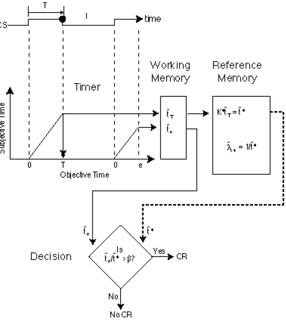
Scalar Expectancy Theory

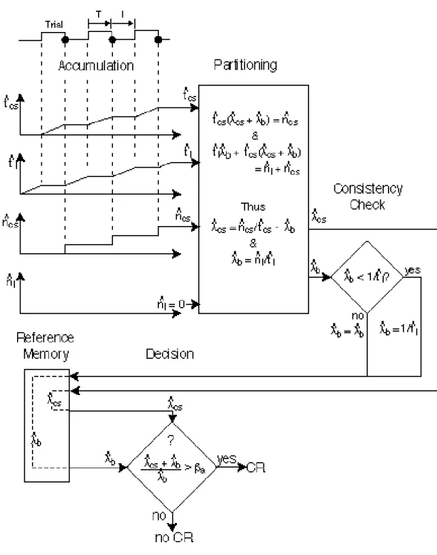
Scalar Expectancy Theory was developed to account for the above aspects of the conditioned response (Gibbon, 1977). It is a model of what we will call the when decision, the decision that determines when the CR occurs in relation to a time mark such as CS onset or offset or the delivery of a previous reinforcement. The basic assumptions of Scalar Expectancy Theory and the components out of which the model is constructed--a timing mechanism, a memory mechanism, sources of variability or noise in the decision variables, and a comparison mechanism adapted to that noise (see Figure 3)-- appear in our explanation of all other aspects of conditioned behavior. The timing mechanism generates a signal, t ˆ _e, which is proportional at every moment to the elapsed duration of the animal’s current exposure to a CS. This quantity in the head is the animal’s measure of the duration of an elapsing interval. The timer is reset to zero by the occurrence of a reinforcement, which marks the end of the interval that began with the onset of the CS. The magnitude of t ˆ _e at the time of reinforcement, t ˆ _T is written to memory through a multiplicative translation variable, k*, whose expected value {E(k*) =K*} is close to but not identically one. Thus, the reinforcement interval recorded in memory, t *ˆ =k * ˆ t _T on average, deviates from the timed value by some (generally small) percentage, which is determined by the extent to which the expected value of K*

deviates from 1. (See Table 1 for a list of the symbols and expressions used, together with their meanings.)

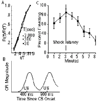
Figure 1. A. Normalized rate of responding as a function of the normalized elapsed interval, for pigeons responding on fixed interval schedules, with inter-reinforcement intervals, T, ranging from 30 to 3,000 s.

R (t)is the average rate of responding at elapsed interval t since the last reinforcement.

R (T)is the average terminal rate of

responding. (Data from Dews, 1970). Plot from Gibbon, 1977, used by permission of the publisher.) B. The time course of the conditioned double blink on a single

representative trial in an experiment in which rabbits were trained with two different US latencies (400 & 900 ms). (Data from Kehoe, Graham-Clarke & Schreurs, 1989) C.

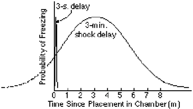
Percent freezing as a function of the interval since placement in the experimental chamber after a single conditioning trial in which rats were shocked 3 minutes after being placed in the chamber. (Data from Fanselow& Stote, 1995 Used with authors’ permission.)

Figure 2. Scalar property: Time scale invariance in the distribution of CRs. A. Responding of three birds on the peak procedure in blocked sessions at reinforcements latencies of 30 s and 50 s (unreinforced CS durations of 90 s and 150 s, respectively). Vertical bars at the reinforcement latencies have heights equal to the peaks of the corresponding distributions.B. The same functions normalized with respect to CS time and peak rate (so that vertical bars would

superpose). Note that although the distributions differ between birds, both in their shape and in whether they peak before or after the reinforcement latency (K* error), they superpose when normalized (rescaled). {Unpublished data from Gibbon}

Table 1: Symbols and Expressions in SET Symbol or

Expression

Meaning

ˆ

t _e time elapsed since CS onset, the subjective measure of an elapsing interval

ˆ

t _T magnitude of t ˆ _e at time of reinforcement, the experienced duration of the CS-US interval

ˆ

t * remembered duration of CS-US interval

k* scaling factor relating t *ˆ to t ˆ _T: t *ˆ =k * ˆ t _T

K * expected value of k*; close to but not equal to 1; fact that value

not equal to 1 explains systematic discrepancy between average experienced duration and average remembered duration, the K *

error ˆ

t _e ˆ t * the decision variable for the when decision, the measure of how similar the currently elapsed interval is to the remembered reinforcement latency

β a decision threshold

T generally, a fixed reinforcement latency. In Pavlovian delay conditioning, the CS-US interval. In a fixed interval operant schedule, the interval between reinforcements

ˆ

λ _cs rate of reinforcement attributed to a CS, the reciprocal of the expected interval between reinforcements

Note: In this and subsequent symbol tables, a hat on a variable indicates that it is a subjective estimate, a quantity in the head representing a physically measurable external variable. Variables without hats are either measurable quantities outside the head, or scaling constants (always symbolized by k’s), or decision thresholds (always symbolized by β).

When the CS reappears (when a new trial begins), t ˆ _e the subjective duration of the currently elapsing interval of CS exposure, is compared to t *ˆ , which is derived by sampling (reading) the remembered reinforce-ment delay in memory. The comparison takes

the form of a ratio, t ˆ _e ˆ t * which we call the decision variable. When this ratio exceeds a threshold, β somewhat less than 1, the animal responds to the CS--provided it has had sufficient experience with the CS to have already decided that it is a reliable predictor of the US (see later section on the acquisition

or whether decision)1. The when decision threshold is somewhat less than 1, because the CR anticipates the US. If, on a given trial, reinforcement does not occur (for example, in the peak procedure, see below), then the conditioned response ceases when this same decision ratio exceeds a second threshold somewhat greater than 1. (The decision to stop responding when the reinforcement interval is past, is not diagrammed in Figure 3, but see Gibbon & Church, 1990).) In short, the animal begins to respond when it estimates the currently elapsing interval to be close to the remembered delay of reinforcement. If it does not get reinforced, it stops responding when it estimates the currently elapsing interval to be sufficiently past the remembered delay. The decision thresholds constitute its criteria for “close” and “past.” Its measure of closeness (or similarity) is the ratio between the currently elapsing and the remembered interval.

The interval timer in SET may be conceived as a clock system (pulse generator) feeding an accumulator (working memory),

1

The decision variable is formally a ratio of random variables and is demonstrably non-normal in most cases. However, the decision rule, te/t* > β is equivalent to te > βt* and the right hand side of this inequality is

approximately normal when t* is normal. When the threshold, β is itself variable, some non-normalilty is induced in the right hand side of the decision rule, introducing some positive skew in this composite variable. Gibbon and his collaborators (Gibbon, 1992; Gibbon, 1981b; Gibbon, Church & Meck, 1984) have discussed the degree of non-normality in this variate in considerable detail. It is shown that a) the mean and variance of the decision variate are readily obtained in closed form, and b) the degree of skew in the composite variable is not large relative to other variance in the system. The behavioral performance often also shows a slight positive skew consistent with the formal analysis.

which continually integrates activity over time. The essential feature of such a mechanism is that the quantity in the accumulator grows as a linear function of time. By contrast, the reference memory system statically preserves the values of past intervals. When accumulation is temporarily halted, for example in paradigms when reinforcement is not delivered and the signal is briefly turned off and back on again after a short period (a gap), the value in the accumulator simply holds through the gap (working memory), and the integrator resumes accumulating when the signal comes back on.

Scalar variability, evident in the constant coefficient of variation in the distribution of the onsets, offsets and peaks of conditioned responding, is a consequence of two fundamental assumptions. The first is that the comparison mechanism uses the ratio of the two values being compared, rather than, for example, their difference. The second is that subjective estimates of temporal durations, like subjective estimates of many other continuous variables (length, weight, loudness, etc.), obey Weber’s law: the difference required to discriminate one subjective magnitude from another with a given degree of reliability is a fixed fraction of that magnitude(Gibbon, 1977; Killeen & Weiss, 1987). What this most likely implies--and what Scalar Expectancy Theory assumes--is that the uncertainty about the true value of a remembered magnitude is proportional to the magnitude. These two assumptions --the decision variable is a ratio and estimates of duration read from memory have scalar variability--are both necessary to explain scale invariance in the distribution of conditioned responses (Church & Gibbon, 1982; Gibbon & Fairhurst, 1994).

Figure 3. Flow diagram for the CR timing or when decision. Two trials are shown, the first reinforced, at T, (filled circle on time line) and the second still elapsing at e. When the first trial is reinforced, the cumulated subjective time, t ˆ _T, is stored in working memory and transferred to reference memory via a multiplicative variable, k* (t *ˆ =k * ˆ t _T ). The decision to respond is based on the ratio of the elapsing interval (in working memory) to the remembered interval (in reference memory). It occurs when this ratio exceeds a threshold (β) close to, but generally less than 1. Note that the reciprocal of t ˆ _T is equal to λ ˆ _cs, the estimated rate of CS reinforcement, which plays a crucial role in the acquisition and extinction decisions described later.

It has recently become clear that much of the observed trial-to-trial variability in

response timing is due to the variability inherent in the signals derived from reading

durations stored in long-term memory, rather than from variability in the timing process that generates inputs to memory . Even when there is only one such comparison duration in memory, a comparison signal t *ˆ , derived from reading that one memory varies substantially from trial to trial. In some paradigms, the standard interval read from memory for comparison to a currently elapsing interval may be based either on a single standard (a single standard experienced repeatedly) or a double standard (two different values experienced in random intermixture). In the 2-standard condition, the comparison value (expectation) recalled from memory is equal to the harmonic mean of the two standards. The trial-to-trial variability in timing performance observed in this 2-standard condition is the same as in a 1-standard condition with a 1-standard equal to the harmonic mean of the standards in the 2-standard condition. The variability in the input to memory is very different in the two conditions, but the output variability is the same. This implies that the trial-to-trial variability in the response latencies is largely due to noise in the memory reading operation rather than variability in the values read into memory. (See Gallistel, in press for a fuller discussion of the evidence for this conclusion.)

The Timing of Appetitive CRs The FI Scallop

An early application of Scalar Expectancy Theory was to the explanation of the "FI scallop” in operant conditioning. An FI schedule of reinforcement delivers reinforcement for the first response made after a fixed interval has elapsed since the delivery of the last reinforcement. When responding on such a schedule, animals pause after each reinforcement, then resume responding after some interval has elapsed. It

was generally supposed that the animal’s rate of responding accelerated throughout the remainder of the interval leading up to reinforcement. In fact, however, conditioned responding in this paradigm, as in many others, is a two-state variable (slow, sporadic pecking versus rapid, steady pecking), with one transition per inter-reinforcement interval (Schneider, 1969). The average latency to the onset of the high-rate state during the post-reinforcement interval increases in proportion to the scheduled reinforcement interval over a very wide range of intervals (from 30s to at least 50 min). The variability in this onset from one interval to the next also increases in proportion to the scheduled interval. As a result, averaging over many inter-reinforcement intervals results in the smooth increase in the average rate of responding that Dews (1970) termed “proportional timing” (Figure 1A). The smooth, almost linear increase in the average rate of responding seen in Figure 1A is the result of averaging across many different abrupt onsets. It could more appropriately be read as showing the probability that the subject will have entered the high-rate state as a function of the time elapsed since the last reinforcement.

The Peak Procedure

The fixed interval procedure only allows one to see the subject’s anticipation of reinforcement. The peak procedure (Catania, 1970; Roberts, 1981) is a discrete-trials modification that enables one also to observe the cessation of responding when the expected time of reinforcement has passed without reinforcement. The beginning of each trial is marked by the illumination of the key (with pigeon subjects) or the extension of the lever (with rat subjects). A response (key peck or lever press) is reinforced only after a fixed interval has elapsed. However, a partial reinforcement schedule is used. On some trials, there is no reinforcement. On these

trials (Peak trials), the CS continues for three or four times the reinforcement latency, allowing the experimenter to observe the cessation of the CR when the expected time of reinforcement has passed. This procedure yielded the data in Figure 2, which come from the unreinforced trials.

The smoothness of the curves in Figure 2 is again an averaging artifact. On any one trial, there is an abrupt onset and an abrupt offset of steady responding (Church, Meck & Gibbon, 1994; Church, Miller, Meck & Gibbon, 1991; Gibbon & Church, 1992). The midpoint of the interval during which the animal responds (the CR interval) is proportionate to reinforcement latency, and so is the average duration of this CR interval. However, there is considerable trial-to-trial variation in the onset and the offset of responding. The curves in Figure 2 are a consequence of averaging across the independently variable onsets and offsets of responding (Church et al., 1994). As in Figure 1A, these curves are more appropriately read as giving the probability that the animal will be responding at a high rate at any given fraction of the reinforcement latency.

The Timing of Aversive CRs Avoidance Responses

The conditioned fear that is manifest in freezing behavior and other indices of a conditioned emotional response is classically conditioned in the operational sense that the reinforcement is not contingent on the animal’s response. Avoidance responses, by contrast, are instrumentally conditioned in the operational sense, because their appearance depends on the contingency that the performance of the conditioned response forestalls the aversive reinforcement. By responding, the subject avoids the aversive stimulus. We stress the purely operational, as

opposed to the theoretical, distinction between classical and instrumental conditioning, because, from the perspective of timing theory, the only difference between the two paradigms is in the events that mark the beginnings of expected and elapsing intervals. In the instrumental case, the expected interval to the next shock is longest immediately after a response, and the recurrence of a response resets the shock clock. Thus, the animal’s response marks the onset of the relevant interval.

The timing of instrumentally conditioned avoidance responses is as dependent on the expected time of aversive reinforcement as the timing of classically conditioned emotional reactions, and it shows the same scale invariance in the mean, and scalar variability around it (Gibbon, 1971, 1972). In shuttle box avoidance paradigms, where the animal gets shocked at either end of the box if it stays too long, the mean latency at which the animal makes the avoidance response increases in proportion to the latency of the shock that is thereby avoided, and so does the variability in this avoidance latency. A similar result is obtained in free-operant avoidance, where the rat must press a lever before a certain interval has elapsed in order to forestall for another such interval the shock that will otherwise occur (Gibbon, 1971, 1972, 1977; Libby & Church, 1974). As a result, the probability of an avoidance response at less than or equal to a given proportion of the mean latency is the same regardless of the absolute duration of the expected shock latency (see, for example, Figure 1 in Gibbon, 1977). Scalar timing of avoidance responses is again a consequence of the central assumptions in Scalar Expectancy Theory--the use of a ratio to judge the similarity between the currently elapsed interval and the expected shock latency, and scalar variability (noise) in the shock latency durations read from memory.

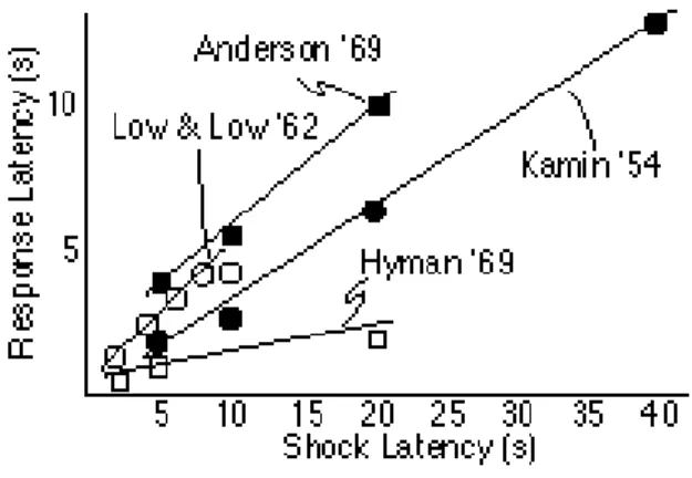
When an animal must respond in order to avoid a pending shock, responding appears long before the expected time of shock. One of the earliest applications of SET (Gibbon, 1971) showed that this early responding in avoidance procedures is nevertheless scalar in the shock delay (Figure 4). According to SET, the expectation of shock is maximal at the experienced latency between the onset of the warning signal and the shock, just as in other paradigms. However, a low decision threshold leads to responding at an elapsed interval equal to a small fraction of the expected shock latency. The result of course is successful avoidance on almost all trials. The low threshold compensates for trial-to-trial variability in the remembered duration of the warning interval. If the the threshold were higher, the subject would more often fail to respond in time to avoid the shock. The low threshold ensures that responding almost always anticipates and thereby forestalls the shock.

Figure 4. The mean latency of the avoidance response as a function of the latency of the shock (CS-US interval) in a variety of cued avoidance experiments with rats (Anderson, 1969; Kamin, 1954; Low & Low, 1962) and monkeys (Hyman, 1969). Note that although the response latency is much shorter than the shock latency, it is nonetheless proportional to the shock latency. The straight lines are drawn by eye {Redrawn with slight

modifications from Gibbon, 1971, by permission of the author and publisher.} The Conditioned Emotional Response

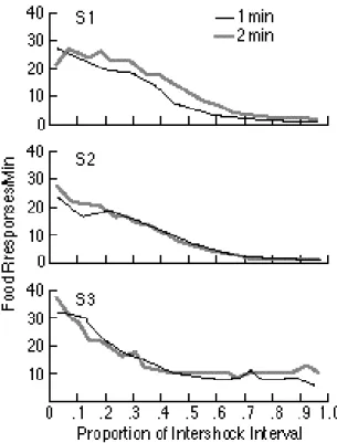
The conditioned emotional response (CER) is the suppression of appetitive responding that occurs when the subject (usually a rat) expects a shock to the feet (aversive reinforcement). The appetitive response is suppressed because the subject freezes in anticipation of the shock (Figure 1C). If shocks are scheduled at regular intervals, then the probability that the rat will stop its appetitive responding (pressing a bar to obtain food) increases as a fraction of the intershock interval that has elapsed. The suppression measure obtained from experiments employing different intershock intervals are superimposable when they are plotted as a proportion of the intershock interval that has elapsed (LaBarbera & Church, 1974-- see Figure 5). Put another way, the degree to which the rat fears the impending shock is determined by how close it is to the shock. Its subjective measure of closeness is the ratio of the interval elapsed since the last shock to the expected interval between shocks--a simple manifestation of scalar expectancy.

The Immediate Shock Deficit

If a rat is shocked immediately after being placed in an experimental chamber (1-5 second latency), it shows very little conditioned response (freezing) in the course of an eight-minute test the next day. By contrast, if it is shocked several minutes after being placed in the chamber, it shows much more freezing during the subsequent test. The longer the reinforcement delay, the more total freezing is observed, up to several minutes (Fanselow, 1986). This has led to the suggestion that in conditioning an animal to fear the experimental context, the longer the

Figure 5. The strength of the conditioned emotional reaction to shock is measured by the decrease in appetitive responding when shock is anticipated: data from three rats. The decrease in responding for a food reward (a measure of the average strength of the fear) is determined by the proportion of the anticipated interval that has elapsed. Thus, the data from conditions using different fixed intershock intervals (1 minute and 2 minutes) are superimposable when normalized. This is time scale invariance in the fear response to impending shock. {Figure reproduced with slight modifications from LaBarbera and Church, 1974, by permission of the authors and publisher.]}

reinforcement latency, the greater the resulting strength of the association (Fanselow, 1986; Fanselow, 1990; Fanselow, DeCola & Young, 1993). This explanation of the immediate shock freezing deficit rests on an ad hoc assumption, made specifically in order to explain this phenomenon. Moreover, it is the opposite of the usual assumption

about the effect of delay on the efficacy of reinforcement, namely, the shorter the delay the greater the effect of reinforcement.

Figure 6. The distribution of freezing behavior in a 10 minute test session following a single training session in which groups of rats were shocked once at different latencies (vertical

arrows) after being placed in the experimental box (and removed 30 s after the shock). The control rats were shocked immediately after being placed in a different box (a different context from the one in which their freezing behavior was observed on the test day). After Fig. 2 in (Bevins & Ayres, 1995).

From the perspective of Scalar Expectancy Theory, the immediate shock freezing deficit is a manifestation of scalar variability in the distribution of the fear response about the expected time of shock. Bevins and Ayres (1995) varied the latency of the shock in one-trial contextual fear conditioning paradigm and showed that the later in the training session the shock is given, the later one observes the peak in freezing behavior and the broader the distribution of this behavior throughout the session (Figure 6). The prediction of the immediate shock deficit follows directly from the scalar variability of the fear response about the moment of peak probability (as evidenced in Figure 5). If the probability of freezing in a test session following training with a 3-minute shock delay is given by the broad normal curve in Figure 7. (cf. freezing data in Figure 1C), then the distribution after a 3-s latency should be 60 times narrower (3-s curve in Figure 7). Thus, the amount of freezing observed during an 8-minute test session following an immediate shock should be negligible in comparison to the amount observed following a shock delayed for 3 minutes.

It is important to note that our explanation of the failure to see significant evidence of fear in the chamber after experiencing short latency shock does not imply that there is no fear associated with that brief delay. On the contrary, we suggest that the subjects fear the shock just as much in the short-latency conditions as in the long-latency condition. But the fear begins and

ends very much sooner; hence, there is much less measured evidence of fear. Because the average breadth of the interval during which the subject fears shock grows in proportion to the remembered latency of that shock, the total amount of fearful behavior (number of seconds of freezing) observed is much greater with longer shock latencies.

Figure 7. Explanation of the immediate shock freezing deficit by Scalar Expectancy Theory: Given the probability-of-freezing curve shown for the 3-minute group (Figure 1C), the scale invariance of CR distributions predicts the very narrow curve shown for subjects shocked immediately (3 s) after placement in the box. Scoring percent freezing during the eight minute test period will show much more freezing in the 3-minute group than in the 3-s group (about 60 times more).

The Eye Blink

The conditioned eye blink is often regarded as a basic or primitive example of a classically conditioned response to an aversive US. A fact well known to those who have directly observed this conditioned response is that the latency to the peak of the conditioned response approximately matches the CS-US latency. Although the response is over literally in the blink of an eye, it is so timed that the eye is closed at the moment when the aversive stimulus is expected. Figure 1B is an interesting example. In the experiment from which this representative plot of a double

blink is taken (Kehoe et al., 1989), there was only one US on any given trial, but it occurred either 400 ms or 900 ms after CS onset, in a trial-to-trial sequence that was random (unpredictable). The rabbit learned to blink twice, once at about 400 ms and then again at 900 ms. Clearly, the timing of the eye blink--the fact that longer reinforcement latencies produce longer latency blinks--cannot be explained by the idea that longer reinforcement latencies produce weaker associations. The fact that the blink latencies approximately match the expected latencies of the aversive stimuli to the eye is a simple indication that the learning of the temporal interval to reinforcement is a foundation of simple classically conditioned responding. Recent findings with this preparation further imply that the learning of the temporal intervals in the protocol is the foundation of the higher order effects called positive and negative patterning and occasion setting (Weidemann, Georgilas & Kehoe, 1999)

The record in Figure 1B does not exhibit scalar variability, because it is a record of the blinks on a single trial. Blinks, like pecks, have, we assume, more or less fixed duration, because they are ballistic responses programmed by the CNS. What exhibits scalar variability from trial to trial is the time at which the CR is initiated. In cases like pigeon pecking, where the CR is repeated steadily for some while, so that there is a stop decision as well as a start decision, the duration of conditioned responding shows the scalar property on individual trials. That is, the interval between the onset of responding and its cessation increases in proportion to the midpoint of the CR interval. In the case of the eye blink, however, where there is only one CR per expected US per trial, the duration of the CR may be controlled by the motor system itself rather than by higher level decision processes. The distribution of these CRs from repeated trials should,

however, exhibit scalar variability. (We are not aware of an analysis of the variability in blink latencies.)

Timing the CS: Discrimination

The acquisition and extinction models to be considered shortly assume that the animal times the durations of the CSs it experiences and compares those durations to durations stored in memory. It is possible to directly test this assumption by presenting CSs of different duration, then asking the subject to indicate by a choice response which of two durations it has just experienced. In other words, the duration of the just experienced CS is made the basis of a discrimination in a successive discrimination paradigm, a paradigm in which the stimuli to be discriminated are presented individually on successive trials, rather than simultaneously in one trial. In the so-called bisection paradigm, the subject is reinforced for one choice after hearing a short duration CS (say, a 2 s CS) and for the other choice after hearing a long duration CS (say, an 8 s CS). After learning the reference durations (the “anchors”) subjects are probed with intermediate durations and required to make classification responses to these.

If the subject uses ratios to compare probe durations to the reference durations in memory, then the point of indifference, the probe duration that it judges to be equidistant from the two reference durations, will be at the geometric mean of the reference durations rather than at their arithmetic mean. SET assumes that the decision variable in the bisection task is the ratio of the similarities of the probe to the two reference durations. The similarity of two durations by this measure is the ratio of the smaller to the larger. Perfect similarity is a ratio of 1:1. Thus, for example, a 5 s probe is more similar to an 8 s probe than to a 2 s probe, because 5/8 is closer to 1

than is 2/5. If, by contrast, similarity were measured by the extent to which the difference between two durations approaches 0, then a 5 s probe would be equidistant (equally similar) to a 2 and an 8 s referent, because 8-5 = 5-2. Maximal uncertainty (indifference) should occur at the probe duration that is equally similar to 2 and 8. If similarity is measured by ratios rather than differences, then the probe is equally similar to the two anchors for T, such that 2/T = T/8 or T=4, the geometric mean of 2 and 8.

As predicted by the ratio assumption in Scalar Expectancy Theory, the probe duration at the point of indifference is in fact generally the geometric mean, the duration at which the ratio measures of similarity are equal, rather than the arithmetic mean, which is the duration at which the difference measures of similarity are equal (Church & Deluty, 1977; Gibbon et al., 1984; see Penney, Meck, Allan & Gibbon, in press for a review and extension to human time discrimination) Moreover, the plots of the percent choice of one referent or the other as a function of the probe duration are scale invariant, which means that the psychometric discrimination functions obtained from different pairs of reference durations superpose when time is normalized by the geometric mean of the reference durations (Church & Deluty, 1977; Gibbon et al., 1984).

Acquisition

The acquisition of responding to the CS

The conceptual framework we propose for the understanding of conditioning is, in its essentials, the decision-theoretic conceptual framework, which has long been employed in psychophysical work, and which has informed SET from its inception. In the psychophysical decision-theoretic

frame-work, there is a stimulus whose strength may be varied by varying relevant parameters. The stimulus might be, for example, a light flash, whose detectability is affected by its intensity, duration and luminosity. The stimulus gives rise through an often complex computational process to a noisy internal signal called the decision variable. The stronger the stimulus, the greater the mean value of this noisy decision variable. The subject responds when the decision variable exceeds a decision threshold. The stronger the stimulus is, the more likely the decision variable is to exceed the decision threshold; hence the more likely the subject is to respond. The plot of the subject’s response probability as a function of the strength of the stimulus (for example, its intensity or duration or luminosity) is called the psychometric function.

In our analysis of conditioning, the conditioning protocol is the stimulus. The temporal intervals in the protocol--including the cumulative duration of the animal’s exposure to the protocol-- are the relevant parameters of the stimulus, as are the reinforcement magnitudes, when they also vary. These stimulus parameters determine the value of a decision variable through a to-be-described computational process, called rate estimation theory (RET). The decision variable is noisy, due to both external and internal sources. The animal responds to the CS when the decision variable exceeds an acquisition threshold. The decision process is adapted to the characteristics of the noise.

The acquisition function in conditioning is equivalent to the psychometric function in a psychophysical task. Its rise (the increasing probability of a response as exposure to the protocol is prolonged) reflects the growing magnitude of the decision variable. The visual stimulus in the example used above gets stronger as the duration of the flash is

prolonged, because the longer a light of a given intensity is continued, the more evidence there is of its presence (up to some limit). Similarly, the conditioning stimulus gets stronger as the duration of the subject’s exposure to the protocol increases, because the continued exposure to the protocol gives stronger and stronger objective evidence that the CS makes a difference in the rate of reinforcement (stronger and stronger evidence of CS-US contingency).

In modeling acquisition, we try to emulate psychophysical modeling by paying closer attention to quantitative results, rather than predicting only the directions of effects. However, our efforts to test models of the simple acquisition process quantitatively are hampered by a paucity of data on acquisition in individual subjects. Most published acquisition curves are group averages. These are likely to contain averaging artifacts. If individual subjects acquire abruptly, but different subjects acquire after different amounts of experience, the averaging across subjects of response frequency as a function of trials or reinforcements will yield a smooth, gradual group acquisition curve, even though acquisition in each individual subject showed abrupt acquisition. Thus, the form of the “psychometric function” (acquisition function) for individual subjects is not well established.

Quantitative facts about the effects of basic variables like partial reinforcement, delay of reinforcement, and the intertrial interval on the rate of acquisition and extinction also have not been as well established as one might suppose, given the rich history of experimental research on conditioning and the long-recognized importance of these parameters2. In recent

2This is in part because meaningful data on

acquisition could not be collected before the advent of

years, pigeon autoshaping has been the most extensively used appetitive conditioning preparation. The most systematic data on rates of acquisition and extinction come from it. Data from other preparations, notably rabbit jaw movement conditioning (another appetitive preparation), the rabbit nictitating membrane preparation (aversive condition-ing) and the conditioned suppression of appetitive responding (CER) preparation (also aversive) appear to be consistent with these data, but do not permit as strong quantitative conclusions.

Pigeon autoshaping is a fully automated variant of Pavlov’s classical conditioning paradigm. The protocol for it is diagrammed in Figure 8A. The CS is the transillumination of a round button (key) on the wall of the experimental enclosure. The illumination of the key may or may not be followed at some delay by the brief presentation of a hopper full of food (reinforcement). Instead of salivating to the stimulus that predicts food, as Pavlov’s dogs did, the pigeon pecks at it. The rate or probability of pecking the key is the measure of the strength of conditioning. As in Pavlov’s original protocol, the CR (pecking) is the same or nearly the same as the UR elicited by the US. In this paradigm, as in Pavlov’s paradigm, the food is delivered at the end of the CS whether or not the subject pecks the key. Thus, it is a classical conditioning paradigm rather than an operant conditioning paradigm. As an automated means for teaching pigeons to peck keys in operant conditioning experiments, it has replaced experimenter-controlled shaping. It is now common practice to condition the

fully automated conditioning paradigms. When experimenter judgment enters into the training in an on-line manner, as is the case when animals are “shaped,” or when the experimenter handles the subjects on every trial (as in most maze paradigms), the skill and attentiveness of the experimenter is an important but unmeasured factor.

pigeon to peck the key by reinforcing key illumination whether or not the pigeon pecks (a Pavlovain procedure) and only then introduce the operant contingency on responding. The discovery that pigeon key pecking--the prototype of the operant response--could be so readily conditioned by a classical (Pavlovian) rather than an operant protocol has cast doubt on the traditional assumption that classical and operant protocols tap fundamentally different association-forming processes (Brown & Jenkins, 1968).

Some well established facts about the acquisition of a conditioned response are:

• The "strengthening" of the CR with extended experience: It takes a number of reinforced trials for an appetitive conditioned response to emerge.

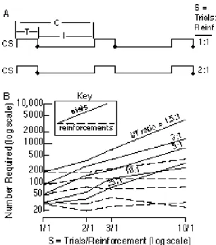
• No effect of partial reinforcement: Reinforcing only some of the CS presentations increases the number of trials required to reach an acquisition criterion in both Palovian paradigms (Figure 8B, solid lines) and operant discrimination paradigms (Williams, 1981). However, the increase is proportional to the thinning of the reinforcement schedule--the average number of trials per reinforcement (the thinning factor). Hence, the required number of reinforcements is unaffected by partial reinforcement (Figure 8B, dashed lines). Thus, the nonrein-forcements that occur during partial reinforcement do not affect the rate of acquisition, defined as the reciprocal of reinforcements to acquisition.

• Effect of the intertrial interval Increasing the average interval between trials increases the rate of acquisition, that is, it reduces the number of reinforcements

required to reach an acquisition criterion (Figure 8B, dashed lines), hence, also trials to acquisition (Figure 8B, solid lines). More quantitatively, reinforce-ments to acquisition are approximately inversely proportional to the I/T ratio (Figures 9 and 10), which is the ratio of the intertrial duration (I) to the duration of a CS presentation (T, for trial duration). If the CS is reinforced on termination (as in Figure 8A), then T is also the reinforcement latency or delay of reinforcement. This interval is also called the CS-US interval or the ISI (for interstimulus interval). The effect of the

I/T ratio on the rate of acquisition is independent of the reinforcement schedule, as may be seen from the fact that the solid lines are parallel in Figure 8B, as are also, of course, the dashed lines.

• Delay of reinforcement: Increasing the delay of reinforcement, while holding the intertrial interval constant, retards acquisition--in proportion to the increase in the reinforcement latency (Figure 11, solid line). Because I is held constant while T is increased, delaying reinforce-ment in this manner reduces the I/T ratio. The effect of delaying reinforcement is entirely due to the reduction in the I/T

ratio. Delay of reinforcement per se does not affect acquisition (dashed line in Figure 11).

• Time scale invariance: When the inter-trial interval is increased in proportion to the delay of reinforcement, delay of reinforcement has no effect on reinforcements to acquisition (Figure 11, dashed line). Increasing the intertrial interval in proportion to the increase in CS duration means that all the temporal intervals in the conditioning protocol are increased by a common scaling factor.

Therefore, we call this important result the time scale invariance of the acquisition process. The failure of partial reinforcement to affect rate of acquisition and the constant coefficient of variation in reinforcements to acquisition (constant vertical scatter about the regression line in Figure 9) are other manifestations of time scale invariance, as will be explained. •Irrelevance of reinforcement magnitude:

Above some threshold level, the amount of reinforcement has little or no effect on the rate of acquisition. Increasing the amount of reinforcement by increasing the duration of food-cup presentation 15-fold does not reduce reinforcements to acquisition. In fact, the rate of acquisition can be dramatically increased by reducing reinforcement duration and adding the time thus saved to the intertrial interval (Figure 12). The intertrial interval, the interval when nothing happens, matters profoundly in acquisition; the duration or magnitude of the reinforcement does not. • Acquisition requires contingency (the

Truly Random Control) When reinforce-ments are delivered during the intertrial interval at the same rate as they occur during the CS, conditioning does not occur (the truly random control, also known as the effect of background conditioning --Rescorla, 1968). The failure of conditioning under these conditions is not simply a performance block, as conditioned responding to the CS after random control training is not observable even with sensitive techniques (Gibbon & Balsam, 1981). The truly random control eliminates the contin-gency between CS and US while leaving the frequency of their temporal pairing unaltered. Its effect on conditioning implies that conditioning is driven by

CS-US contingency, not by the temporal pairing of CS and US.

• Effect of signaling 'background' rein-forcers. In the truly random control procedure, acquisition to a target CS does occur if another CS precedes (and thereby signals) the 'background' reinforcers (Durlach, 1983). These signaled forcers are no longer background rein-forcers if, by a background reinforcer, one means a reinforcer that occurs in the presence of the background alone.

Figure 8. A. Time lines showing the variables that define a classical (Pavlovian)

conditioning protocol--the duration of a CS presentation (T), the duration of the intertrial interval (I ), and the reinforcement schedule , S(trials/reinforcement). The US

(reinforcement) is usually presented at the termination of the CS (black dots). For reasons shown in Figure 12, the US may be treated as a point event, an event whose duration can be ignored. The sum of T and I is C, the duration of the trial cycle. B.Trials to acquisition (solid lines) and reinforcements to acquisition (dashed lines) in pigeon

autoshaping, as a function of the

reinforcement schedule and theI/Tratio. Note that the solid and dashed lines come in pairs, with the members of a pair joined at the 1/1 value of S, because, with that schedule (continual reinforcement), the number of reinforcements and number of trials are identical. The acquisition criterion was at least one peck on three out of four consecutive presentations of the CS. (Reanalysis of data in Fig. 1 of Gibbon, Farrell, Locurto, Duncan & Terrace, 1980)

1000 100 10 1 .1 1 10 100 1000

B&P 79 B&J 68 G&W, 71, 73 G et al 75 G et al VC G et al FC G et al 80 R et al 77 T et al 75 T 76a T 76b W & McC 74 Regression

I/T

Reinforcements to Acquisition

Figure 9. Reinforcements to acquisition as a function of the I/T ratio. (double logarithmic coordinates). The data are from12

experiments in several different laboratories, as follows: B&P 79 = Balsam & Payne, 1979; B&J 68 = Brown & Jenkins, 1968; G&W,71,73 = Gamzu & Williams, 1971, 1973); G et al 75 = Gibbon, Locurto & Terrace, 1975; G et al VC = Gibbon, Baldock, Locurto, Gold & Terrace, 1977 Variable C; G et al FC = Gibbon et al., 1977 Fixed C; G et al 80 = Gibbon et al., 1980; R et al 77 = Rashotte, Griffin & Sisk, 1977; T et al 75 = Terrace, Gibbon, Farrell & Baldock, 1975; T76a = Tomie, 1976a; T76b = Tomie, 1976b; W & McC74 = Wasserman &

McCracken, 1974.

Figure 10. Selected data showing the effect of I/T ratio on the rate of eye blink conditioning in the rabbit, where I is the estimated amount of exposure to the experimental apparatus per CS trial (time when the subject was outside the apparatus not counted). We used 50% CR frequency as the acquisition criterion in deriving these data from published group acquisition curves. S&G, 1964 =

Schneiderman & Gormezano(1964) 70-trials per session, session length roughly half an hour,Ivaried randomly with mean of 25 s. B&T, 1965 = Brelsford & Theios (1965) single-session conditioning, Is of 45, 111, and 300 s, session lengths increased withI(1.25 & 2 hrs for data shown). We do not show the 300 s data because those sessions lasted about 7 hours. Fatigue, sleep, growing restiveness, etc. may have become an important factor. Lenvinthal, et al., 1985 = Levinthal, Tartell, Margolin & Fishman, 1985, one trial per 11 minute (660-s) daily session. None of these studies was designed to study the effect ofI/Tratio, so the plot should be treated with caution. Such studies are clearly desirable--in this and other standard conditioning paradigms.

We have presented data from pigeon autoshaping to illustrate the basic facts of acquisition (Figures 8, 9, 11 and 12), because the most extensive and systematic

quantitative data come from experiments using that paradigm. However, the same effects (and surprising lack of effects) seem to be apparent in other classical conditioning paradigms. For example, partial reinforce-ment produces little or no increase in reinforcements to acquisition in a wide variety of paradigms (see citations in Table 2 of Gibbon et al., 1980; also Holmes & Gormezano, 1970; Prokasy & Gormezano, 1979); whereas, lengthening the amount of exposure to the experimental apparatus per CS trial increases the rate of conditioning in the rabbit nictitating membrane preparation by almost two orders of magnitude (Kehoe & Gormezano, 1974; Levinthal et al., 1985; Schneiderman & Gormezano, 1964--see Figure 10). Thus, it appears to be generally true that varying the I/T ratio has a much stronger effect on the rate of acquisition than does varying the degree of partial reinforcement, regardless of the conditioning paradigm used.

Figure 11. Reinforcements to acquisition as a function of delay of reinforcement (T), with the (average) intertrial interval (I) fixed (solid line) or varied in proportion to delay of reinforcement (dashed line). [Replot (by interpolation) of data in Gibbon et al.,

(1977)]. For the solid line, the intertrial interval was fixed at I=48 s. For the dashed

line, the I/T ratio was fixed at 5.

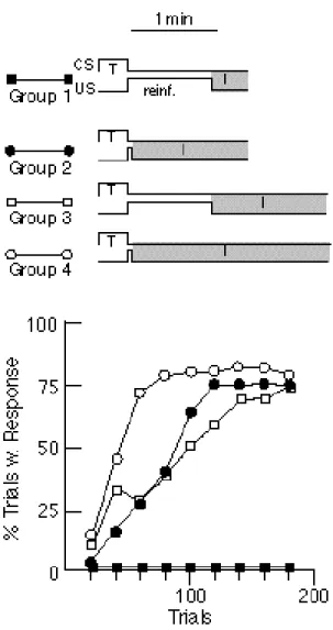
Figure 12.Effect on rate of acquisition of allocating time either to reinforcement or to the intertrial interval(I). Groups 1 & 2 had the same duration of the trial cycle (T + I +

reinforcement time), but Group 2 had its reinforcement duration reduced by a factor of 15 (from 60 to 4 s). The time thus saved was added to the intertrial interval. Group 2 acquired, while Group 1 did not. Groups 3 & 4 had longer (and equal) cycle durations. Again, a 56s interval was used either for reinforcement (Group 3) or as part of the intertrial interval (Group 4). Group 4

acquired most rapidly. Group 3, which had the same I/T ratio as Group 2, acquired no faster than Group 2, despite getting 15 times more access to food per reinforcement. (Replotted from Figs. 1 & 2 in Balsam & Payne, 1979 by permission of the authors and publisher).

It also appears to be generally true that in both appetitive and aversive conditioning paradigms, varying the magnitude or intensity of reinforcement has little effect on the rate of acquisition. Increasing the magnitude of the water reinforcement in rabbit jaw-movement conditioning 20-fold has no effect on the rate of acquisition (Sheafor & Gormezano, 1972). Turning to aversive conditioning, Annau and Kamin (1961) examined the effect of shock intensity on the rate at which fear-induced suppression of appetitive responding is acquired. The groups receiving the three highest intensities (0.85, 1.55 & 2.91 ma) all went from negligible levels of suppression to complete suppression on the second day of training (between trials 4 and 8). The group receiving the next lower shock intensity (0.49 ma) showed less than 50% suppression asymptotically. Kamin (1969a) later examined the effect of two levels of shock intensity on the rate at which CERs to a light CS and a noise CS were acquired. He used 1 ma, which is the usual level in CER experiments, and 4 ma, which is a very intense shock. The 1 ma groups crossed the 50% median suppression criterion between trials 4 and 5, while the 4 ma groups crossed this criterion between trials 3 and 4. Thus, varying shock intensity from the minimum that sustains a vigorous fear response up to very high levels has little effect on the rate of CER acquisition.

The lack of an effect of US magnitude or intensity on the number of reinforcements required for acquisition is counterintuitive and merits further investigation in a variety of

paradigms. In such investigations, it will be important to show data from individual subjects to avoid averaging artifacts. For the same reason, it will be important not to bin the responses by session or number of trials, etc. What one wants is the real-time record of responding. Finally, it will be important to distinguish between the asymptote of the acquisition function and the location of its rise, defined as, the number of reinforcements required to produce, for example, a half-maximal rate of responding. At least from a psychophysical perspective, only the latter measure is relevant to determining the rate of acquisition. In psychophysics, it has long been recognized that it is important to distinguish between the location of the psychometric function along the x-axis (in this case, number of reinforcements), on the one hand, and the asymptote of the function, on the other hand. The location of the function indicates the underlying rate or sensitivity, while its asymptote reflects performance factors. The same distinction is used in pharmacology: the location (dose required for) the half-maximal response indicates affinity, while the asymptote indicates performance factors such as the number of receptors available for binding.

We do not claim that reinforcement magnitude is unimportant in conditioning. As we will emphasize later on, it is a very important determinant of preference. It is also an important determinant of the asymptotic level of performance. And, if the magnitude of reinforcement varied depending on whether the reinforcement was delivered during the CS or during the background, we would expect magnitude to affect rate of acquisition as well. A lack of effect on rate of acquisition is observed (and, on our analysis, expected) only when there are no background reinforcements (the usual case in simple conditioning) or when the magnitude of background reinforcements is the same as the

background reinforcements equals the magnitude of CS reinforcements (the usual case when there is background conditioning).

Rate Estimation Theory

From a timing perspective, acquisition is a consequences of decisions that the animal makes about whether to respond to a CS. Our models for these decisions are adapted from Gallistel's earlier account (Gallistel, 1990, 1992a, b), which we will call Rate Estimation Theory (RET). In our acquisition model, the decision to respond to the CS in the course of conditioning is based on the animal's growing certainty that the CS has a substantial effect on the rate of reinforce-ment. In simple conditioning, this certainty appears to be determined by the subject’s estimate of the maximum possible value for the rate of background reinforce-ment given its experience of the background up to a given point in conditioning. Its estimate of the upper limit on what the rate of background reinforcement may be decreases steadily as conditioning progresses, because the subject never experiences a background reinforcement (in simple conditioning). The subject’s estimate of the rate of CS reinforcement, by contrast, remains stable, because the subject gets reinforced after every so many seconds of exposure to the CS. The decision to respond is based on the ratio of these rate estimates, as shown in Figure 13. This ratio gets steadily larger as conditioning pro-gresses, because the upper limit on the background rate gets steadily lower. It should already be apparent why the amount of background exposure is so important in acquisition. It determines how rapidly the estimate for the background rate of reinforcement diminishes.

The ratio of two estimates for rates of reinforcement is equivalent to the ratio of two estimates of the expected interval between

reinforcements (the interval-rate duality principle). Thus, any model couched in terms of rate ratios can also be couched in terms of the ratios of the expected intervals between events. When couched in terms of the expected intervals between reinforce-ments, the RET model of acquisition is as follows: Because the subject never experiences a background reinforcement in standard delay conditioning (after the hopper training), its estimate of the interval between background reinforcements gets longer in proportion to the duration of its unreinforced exposure to the background. By contrast, its estimate of the interval between reinforce-ments when the CS is on remains constant, because it gets reinforced after every T seconds of CS exposure. Thus, the ratio of the two expected intervals gets steadily greater as conditioning progresses. When this ratio exceeds a decision threshold, the animal begins to respond to the CS

The interval-rate duality principle means that the decision variables in SET and RET are the same kind of variables. Both decision variables are equivalent to the ratio of two estimated intervals. Rescaling time does not affect these ratios, which is why both models are time scale invariant. This time-scale invariance is, we believe, unique to timing-based models of conditioning with decision variables that are ratios of estimated intervals. It provides a simple way of discriminating experimentally between these models and associative models. There are, for example, many associative explanations for the trial-spacing effect (Barela, 1999, in press), which is the strong effect that lengthening the intertrial interval has on the rate of acquisition (Figures 9 & 10). To our knowledge, none of them is time-scale invariant. That is, in none of them is it true that the magnitude of the trial-spacing effect is determined simply by the relative amounts of exposure to the CS and to the background

alone in the protocol (Figure 11). The explanation of the trial-spacing effect given by Wagner’s (1981) “sometimes opponent process (SOP) model, for example, depends on the rates at which stimulus traces decay from one state of activity to another. The size of the predicted effect of trial spacing will not be the same for protocols that have the same proportion of CS exposure to intertrial interval and differ only in their time scale, because longer time scales will lead to more decay. This time-scale dependence is seen in the predictions of any model that assumes intrinsic rates of decay (of, for example, stimulus traces, as in Sutton & Barto, 1990) or any model that assumes that experience is carved into trials (Rescorla & Wagner, 1972, for example).

Rate Estimation Theory offers a model of acquisition that is distinct from, albeit similar in inspiration to, the model proposed by Gibbon and Balsam (1981). The idea underlying both models is that the decision whether to respond to a CS in the course of conditioning depends on a comparison of the estimated rate of CS reinforcement to the estimated rate of background reinforcement (cf. Miller’s Comparator Hypothesis -- Cole, Barnet & Miller, 1995a; Miller, Barnet & Grahame, 1992). In our current proposal, RET incorporates scalar variability in the interval estimates, just as SET did in estimating the point within the CS at which responding should be seen. In RET, however, two new principles are introduced: First, the relevant time intervals are cumulated across successive occurrences of the CS and across successive intervals of background alone. The total cumulated time in the CS and the total cumulated exposure to the background are integrated throughout a session and even across sessions, provided no change in rates of reinforcement is detected.

Cumulations over separated occurrences of a signal have previously been shown to be relevant to performance when no reinforcers intervene at the end of successive CSs. These are the "gap" (Meck, Church & Gibbon, 1985) and "split trials" (Gibbon & Balsam, 1981) experiments, which show that subjects do, indeed, cumulate successive times over successive occurrences of a signal. However, the cumulations proposed in RET extend over much greater intervals (and much greater gaps) than those employed in the just cited experiments. This raises the important question of how accumulation without (practical) limit may be realized in the brain. We conjecture that the answer to this question may be related to the question of the origin of the scalar variability in remembered magnitudes. Pocket calculators accumulate magnitudes (real numbers) without practical limit, but not with a precision that is independent of magnitude. What is fixed is the number of significant digits, hence, the percent accuracy with which a magnitude (real number) may be specified. The scalar noise in remembered magnitudes gives them the same property: a remembered magnitude is only specified to within plus or minus a certain percentage of its “true” value, and the decision process is adapted to take account of this. Scalar uncertainty about the value of an accumulated magnitude may be inherent in any scheme that permits accumulation without practical limit -- for example through a binary cascade of accumulators as suggested by Gibbon. Malapani, Dale & Gallistel (1997) Quantitative details on such a model are in preparation by Killeen (personal communication). Our point is that scalar uncertainty about the value of a quantity may be inherent in a scale invariant computational device, a device capable of working with magnitudes of any scale.