FEDERAL RESERVE BANK OF SAN FRANCISCO WORKING PAPER SERIES
Have We Underestimated the Likelihood and Severity
of Zero Lower Bound Events?
Hess Chung
Federal Reserve Board of Governors Jean-Philippe Laforte
Federal Reserve Board of Governors David Reifschneider
Federal Reserve Board of Governors John C. Williams
Federal Reserve Bank of San Francisco
January 2011
Working Paper 2011-01
http://www.frbsf.org/publications/economics/papers/2011/wp11-01bk.pdf
The views in this paper are solely the responsibility of the authors and should not be interpreted as reflecting the views of the Federal Reserve Bank of San Francisco or the Board of Governors of the Federal Reserve System.
Have We Underestimated the Likelihood and Severity
of Zero Lower Bound Events?
Hess Chung Jean-Philippe Laforte
David Reifschneider John C. Williams*
January 7, 2011
Abstract
Before the recent recession, the consensus among researchers was that the zero lower bound (ZLB) probably would not pose a significant problem for monetary policy as long as a central bank aimed for an inflation rate of about 2 percent; some have even argued that an appreciably lower target inflation rate would pose no problems. This paper reexamines this consensus in the wake of the financial crisis, which has seen policy rates at their effective lower bound for more than two years in the United States and Japan and near zero in many other countries. We conduct our analysis using a set of structural and time series statistical models. We find that the decline in economic activity and interest rates in the United States has generally been well outside forecast confidence bands of many empirical macroeconomic models. In contrast, the decline in inflation has been less surprising. We identify a number of factors that help to account for the degree to which models were surprised by recent events. First, uncertainty about model parameters and latent variables, which were typically ignored in past research, significantly increases the probability of hitting the ZLB. Second, models that are based primarily on the Great Moderation period severely understate the incidence and severity of ZLB events. Third, the propagation mechanisms and shocks embedded in standard DSGE models appear to be insufficient to generate sustained periods of policy being stuck at the ZLB, such as we now observe. We conclude that past estimates of the incidence and effects of the ZLB were too low and suggest a need for a general reexamination of the empirical adequacy of standard models. In addition to this statistical analysis, we show that the ZLB probably had a first-order impact on macroeconomic outcomes in the United States. Finally, we analyze the use of asset purchases as an alternative monetary policy tool when short-term interest rates are constrained by the ZLB, and find that the Federal Reserve’s asset purchases have been effective at mitigating the economic costs of the ZLB. In particular, model simulations indicate that the past and projected
expansion of the Federal Reserve's securities holdings since late 2008 will lower the unemployment rate, relative to what it would have been absent the purchases, by 1½ percentage points by 2012. In addition, we find that the asset purchases have probably prevented the U.S. economy from falling into deflation.
* Chung, Laforte, and Reifschneider: Board of Governors of the Federal Reserve; Williams: Federal Reserve Bank of San Francisco. We thank Justin Weidner for excellent research assistance. The opinions expressed are those of the authors and do not necessarily reflect views of the Federal Reserve Bank of San Francisco, the Board of Governors of the Federal Reserve System, or anyone else in the Federal Reserve System.
I. Introduction
The zero lower bound (ZLB) on nominal interest rates limits the ability of central banks to add monetary stimulus to offset adverse shocks to the real economy and to check unwelcome disinflation. The experience of Japan in the 1990s motivated a great deal of research on both the macroeconomic consequences of the ZLB and on monetary policy strategies to overcome these effects. Economic theory has provided important insights about both the dynamics of the economy in the vicinity of the ZLB and possible policy strategies for mitigating its effects. But theory alone cannot provide a quantitative assessment of the practical importance of the ZLB threat, which depends critically on the frequency and degree to which the lower bound constrains the actions of the central bank as it seeks to stabilize real activity and inflation, thereby
impinging on the unconstrained variability and overall distribution of the nominal funds rate that would otherwise arise. These factors in turn depend on the expected magnitude and persistence of adverse shocks to the economy; the dynamic behavior of real activity, inflation, and
expectations; and the monetary policy strategy followed by the central bank, including its inflation target. (The latter factor plays a key role in ZLB dynamics, because the mean of the unconstrained distribution of the nominal funds rate equals the inflation target plus the economy’s equilibrium real short-term rate of interest.) The quantitative evaluation of these factors requires one to use a model of the economy with sound empirical foundations.
Previous research was generally sanguine about the practical risks posed by the ZLB, as long as the central bank did not target too low an inflation rate. Reifschneider and Williams (2000) used stochastic simulations of the Federal Reserve’s large-scale rational-expectations macroeconometric model, FRB/US, to evaluate the frequency and duration of episodes when policy was constrained by the ZLB. They found that if monetary policy followed the
prescriptions of the standard Taylor (1993) rule with an inflation target of 2 percent, the federal funds rate would be near zero about 5 percent of the time and the “typical” ZLB episode would last four quarters. Their results also suggested that the ZLB would have relatively minor effects on macroeconomic performance under these policy assumptions. In addition, they found that monetary policy rules with larger responses to output and inflation than the standard Taylor rule encountered the ZLB more frequently, with relatively minor macroeconomic consequences as long as the inflation target did not fall too far below 2 percent. Other studies reported similar findings although they, if anything, tended to find even smaller effects of the ZLB; see, for
example, Coenen (2003), Schmitt-Grohe and Uribe (2007), and other papers in the reference list. Finally, research in this area suggested that monetary policies could be crafted that would greatly mitigate any effect of the ZLB. Proposed strategies to accomplish this goal included responding more aggressively to economic weakness and falling inflation, or promising to run an easier monetary policy for a time once the ZLB is no longer binding (see Reifschneider and Williams (2002) and Eggertsson and Woodford (2003) and references therein).
The events of the past few years call into question the reliability of those analyses. The federal funds rate has been at its effective lower bound for two years, and futures data suggest that market participants currently expect it to remain there until late 2011. The current episode thus is much longer than those typically generated in the simulation analysis of Reifschneider and Williams (2000). The same study suggested that recessions as deep as what we are now experiencing would be exceedingly rare—on the order of once a century or even less frequent. Of course, recent events could be interpreted as just bad luck—after all, five hundred year floods do eventually happen. Alternatively, they could be flashing a warning sign that previous
estimates of ZLB effects significantly understated the inherent volatility of the economy that arises from the interaction of macroeconomic disturbances and the economy’s dynamics.
The goal of this paper is to examine and attempt to answer three key questions regarding the frequency and severity of ZLB episodes using a range of econometric models, including structural and time series models. First, how surprising have recent events been and what lessons do we take for the future in terms of the expected frequency, duration, and magnitude of ZLB episodes? Second, how severely did the ZLB bind during the recent crisis? And, third, to what extent have alternative monetary policy actions been effective at offsetting the effects of the ZLB in the current U.S. situation?
In examining these questions, we employ a variety of structural and statistical models, rather than using a single structural model as was done in most past research. Research on the ZLB has generally focused on results from structural models because many of the issues in this field have monetary policy strategy and expectational dynamics at their core. For example, studies have typically employed structural models run under rational expectations to assess expected macro performance under, say, different inflation targets or under price-level targeting in order to ensure consistency between the central bank’s actions and private agents’ beliefs. In this paper, we use two empirical macroeconomic models developed at the Board of Governors—
one a more traditional large-scale model and the other an optimization-based dynamic stochastic general equilibrium model—to analyze the extent that the ZLB is likely to constrain policies. In addition, we use the Smets and Wouters (2007) estimated DSGE model. Because these models have strong empirical foundations, they should provide informative quantitative estimates of the risks posed by the ZLB.
However, a potential drawback to using structural models to quantify the likelihood of the risks confronting policymakers is that such models impose stringent constraints and priors on the data, and such restrictions may inadvertently lead to flawed empirical characterizations of the economy. In particular, they are all constructed to yield “well-behaved” long-run dynamics, as long as the monetary policy rule satisfies certain conditions such as the Taylor principle, and as long as the fiscal authorities (explicitly or implicitly) pursue stable policies that, say, target a fixed debt-to-GDP ratio. In addition, these models tend to abstract from structural change and generally assume that the parameters and the shock processes are constant over time and known by policymakers. As a result of these features, structural models may significantly understate the persistence of episodes of low real interest rates, because they implicitly assume that the
medium- to long-run equilibrium real interest rate—a key factor underlying the threat posed by the ZLB—is constant.1 This is because the asymmetric nature of the ZLB implies that low frequency variation in the equilibrium real interest rate raises the overall probability of hitting the ZLB, all else equal.
Because of these potential limitations of structural models, we include in our analysis three statistical models that impose fewer theoretical constraints on the data and allow for a wider set of sources of uncertainty. One is a vector autoregression model with time-varying parameters (TVP-VAR); the second is a model that allows for unit-root behavior in both
potential output growth and the equilibrium real interest rate (Laubach-Williams 2003); and the third is a univariate model that allows for GARCH error processes. In selecting these statistical models, one of our aims is to use models that arguably provide more scope than structural
1 Whether or not real interest rates are stationary is, admittedly, not obvious. Ex post measures for the United States display no clear trend over the past sixty years, and the fact that U.S. real short-term rates were on average low during the 1970s, and high during the 1980s, is in part an artifact of excessively loose monetary policy in the former period and corrective action during the latter period. But phenomena such as the persistent step-down in Japanese output growth since the early 1990s, the global savings glut of the past decade, and secular trends in government indebtedness illustrate that there are many reasons to view the equilibrium real interest rate as a series that can shift over time.
models do for taking into account uncertainty about the range and persistence of movements in the equilibrium real interest rate.
In summary, our findings are as follows. We find that the decline in economic activity and interest rates in the United States has generally been well outside forecast confidence bands of many empirical macroeconomic models. In contrast, the decline in inflation has been less surprising. This underestimation of the risk of the ZLB can be traced to a number of sources. For one, uncertainty about model parameters and latent variables, which were typically ignored in past research, significantly increases the probability of hitting the ZLB. Second, models that are based primarily on the Great Moderation period severely understate the incidence and severity of ZLB events. Third, the propagation mechanisms and shocks embedded in standard DSGE models appear to be insufficient to generate sustained periods of policy being stuck at the ZLB, such as we now observe. We conclude that past estimates of the incidence and effects of the ZLB were too low and suggest a need for a general reexamination of the empirical adequacy of standard models. In addition to this statistical analysis, we show that the ZLB probably had a first-order impact on macroeconomic outcomes in the United States, based on simulations of the FRB/US model (see also Williams 2009). Finally, we analyze the use of asset purchases as a monetary policy tool when short-term interest rates are constrained by the ZLB, and find that the Federal Reserve’s asset purchases have been effective at mitigating the economic costs of the ZLB. In particular, model simulations indicate that the past and projected expansion of the Federal Reserve's securities holdings since late 2008 will lower the unemployment rate, relative to what it would have been absent the purchases, by 1½ percentage points by 2012. In addition, we find that the asset purchases have probably prevented the U.S. economy from falling into deflation.
II. Models and methodological issues
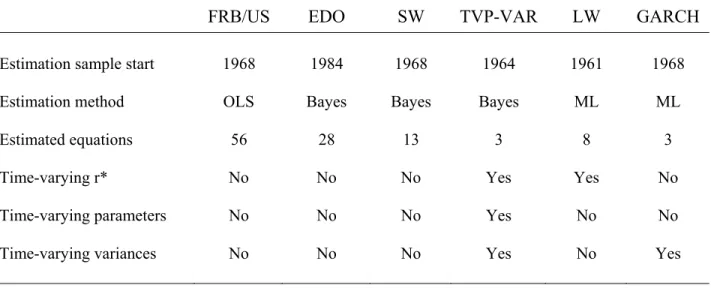
As noted, we use six different models to evaluate the likely incidence of encountering the ZLB. Each of these models is “off the shelf” in that we have taken models already in use at the Federal Reserve or that are well-established in the academic literature. In this section, we provide brief descriptions of the models and references for more detailed information. Table 1 provides a summary of the key features of the models.
FRB/US
The FRB/US model is a large-scale estimated model of the U.S. economy with a detailed treatment of the monetary transmission mechanism. We include the FRB/US model because it has good empirical foundations and has long been used at the Federal Reserve for forecasting and policy analysis. In addition, FRB/US has the advantage of having been used in previous analyses of the ZLB. Although it is not a DSGE model, the main behavioral equations are based on the optimizing behavior of forward-looking households and firms subject to costs of
adjustment. The model displays sluggish adjustment of real activity and inflation in response to shocks (see Brayton et al. 1997 for details).
We assume rational expectations for those parts of our analysis where we explore the macroeconomic effects of substantial changes in monetary policy, such as alternative policy rules or the initiation of large-scale asset purchases. In forecasting exercises, however, we simulate the model using the expectational assumption commonly used at the Fed for this type of work. Under this assumption, agents base their expectations on the forecasts of a small VAR model rather than the full FRB/US model. This approach has the virtue of computational simplicity; it also has a proven track record in forecasting.
Another noteworthy aspect of the FRB/US projections presented in this paper concerns the extrapolation of shocks and exogenous variables. Although shocks to behavioral equations are assumed to be serially uncorrelated with mean zero in the estimation of the model, we do not follow the standard approach used with the other models and set the baseline projected values of the stochastic innovations to zero. Instead, we extrapolate these shocks at their weighted
average value over the preceding sixty quarters, using weights that decline geometrically at a rate of 1 percent per quarter. Analysis at the Federal Reserve indicates that this type of intercept-adjustment procedure—which has been the standard approach to forecasting with FRB/US since the inception of the model in the mid-1990s—increases real-time predictive accuracy. As for exogenous variables, again we follow standard practice in FRB/US forecasting and extrapolate these series using simple univariate time-series equations.
SW (Smets-Wouters)
Our second model is a slightly modified version of the DSGE model developed by Smets and Wouters (2007) (SW hereafter). We made three minor modifications made to the original
model and refer readers to the original paper for a more complete description of the model. The first modification is that we assume that the monetary policy shocks are independently and normally distributed. Second, we replace the measure of the output gap in SW (2007), which is based on a definition of potential output consistent with an equilibrium where nominal rigidities are absent, by a production function-based measure (see Kiley 2010). Finally, we follow the approach of Justiniano, Primiceri, and Tambalotti (2010) and include purchases of consumer durables in the investment series as opposed to the consumption series.
EDO (Estimated Dynamic Optimization-based model)
The EDO model is a DSGE model of the US economy developed and used at the Board of Governors for forecasting and policy analysis; see Chung, Kiley and Laforte (2010) for documentation on the current version of the model, and Edge, Kiley and Laforte (2008) for additional information. Like FRB/US and the SW model, EDO has strong empirical
foundations. And although the model has not been in service long enough at the Federal Reserve to compile a reliable track record, pseudo real-time forecasting exercises suggest that it has good forecasting properties.
EDO builds on the Smets and Wouters (2007) model. Households have preferences over nondurable consumption services, durable consumption services, housing services, and leisure and feature internal habit in each service flow. Production in the model takes place in two distinct sectors that experience different stochastic rates of technological progress—an assumption that allows the model to match the much faster rate of growth in constant dollar-terms observed for some expenditure components, such as nonresidential investment. As a result, growth across sectors is balanced in nominal, rather than real, terms. Expenditures on nondurable consumption, durable consumption, residential investment, nonresidential investment are modeled separately while the remainder of aggregate demand is represented by an exogenous stochastic process.
Wages and prices are sticky in the sense of Rotemberg (1982), with indexation to a weighted average of long-run inflation and lagged inflation. A simple estimated monetary policy reaction function governs monetary policy choices. The exogenous shock processes in the model include the monetary policy shock; the growth rates of economy-wide and investment-specific technologies; financial shocks, such as a stochastic economy-wide risk premium and stochastic
risk premia that affect the intermediaries for consumer durables, residential investment, and nonresidential investment; shocks to autonomous aggregate demand; and price and wage markup shocks.
The model is estimated using Bayesian methods over the sample period 1984Q4 to 2009Q4. Accordingly, the model’s estimates are guided almost entirely by the Great Moderation period. The data used in estimation include the following: real GDP; real consumption of
nondurables and services excluding housing; real consumption of durables; real residential investment; real business investment; aggregate hours worked in the nonfarm business sector (per capita); PCE price inflation; core PCE price inflation; PCE durables inflation; compensation per hour divided by GDP price index; and the federal funds rate. Each expenditure series is measured in per capita terms, using the (smoothed) civilian non-institutional population over the age of 16. We remove a very smooth trend from hours per capita prior to estimation.
TVP-VAR
The specification of the TVP-VAR (time-varying parameter vector autoregression) model closely follows Primiceri (2005). The VAR model contains a constant and two lags of the four-quarter change in the GDP price index, the unemployment rate, and the 3-month Treasury bill rate. Let ܺ௧ denote the column vector consisting of these variables, ordered as listed. The system obeys
(1.1) 0 2 1
1
t t t t t s t t
s
A X A A X B
where ܣ௧ is lower triangular and each non-zero element of the A matrices follows an
independent Gaussian unit-root process. Consequently, both the equilibrium real interest rate and the variances of the shocks are time-varying. The matrix ܤ௧ is diagonal and the logarithm of an entry on the diagonal follows an independent Gaussian unit-root process, i.e., the volatility of structural shocks is stochastic. Estimation is Bayesian, with the prior constructed as in Primiceri (2005), using a 40 quarter training window starting in 1953Q3.2
2 The prior setting is identical to Primiceri (2005), with one exception: we have set the prior mean of the covariance matrix for innovations to the log-variances substantially higher than in that paper. Specifically, the prior mean is [0.05, 0.05, 0.001], versus [0.0004, 0.0004, 0.0004] with the original prior. Relative to the original, this prior favors drift in volatilities more so than in VAR coefficients. The estimation algorithm also follows Primiceri (2005) exactly, except that we use the approach of Jacquier, Polson and Rossi (1994) to draw the log-variance states. The MCMC sample was 20000 draws, following a burn-in run of 10000 iterations.
Laubach-Williams
The Laubach-Williams (LW) model includes estimated equations for the output gap, core PCE price inflation, the funds rate, and relative non-oil import and oil prices. (See Laubach and Williams, 2003). Potential GDP, its growth rate, and the equilibrium real interest rate are all nonstationary unobserved latent variables. The other parameters of the model, including those describing the variances of the shock processes, are assumed to be constant.3 We estimate the LW model by maximum likelihood using the Kalman filter using data starting in 1961.4 Unlike FRB/US and EDO, the LW model implicitly assumes adaptive expectations, features very gradual dynamic responses to shocks, and includes permanent shocks to the equilibrium real interest rate.
GARCH model
We estimate univariate GARCH models of the 3-month Treasury bill rate, the inflation rate of the GDP price index, and the unemployment rate. Specifically, each series is assumed to follow an auto-regressive process of order two
(1.2) xt c a x1 t1a x2 t2et,
where the conditional variance of the innovation, et, is given by
(1.3) 2 2 2
1 1
p
t i t i j t j
i j
G A e
and each equation is estimated subject to the constraints (1.4)
1 1
1, >0, 0, 0 p
i j i j
i j
G A G A
.
3 In order to conduct stochastic simulations of the model, we append AR(1) equations (without constants) for relative oil and nonoil import prices to the model and estimate the additional parameters jointly with the other model parameters.
4 The Kalman gain parameters for the growth rate of potential output and the latent variable that influences the equilibrium real interest rate are estimated using Stock and Watson’s (1998) median unbiased estimator as described in Laubach and Williams (2003). We do not incorporate uncertainty about these gain parameters in our analysis in this paper. Doing so would imply even greater uncertainty about interest rates and raise the probability of hitting the ZLB.
The lag structure of the GARCH model was selected on the basis of the Bayesian information criterion over the sample 1968q1-2007q4.5 See Engle (2001) for further details on the estimation of GARCH models.
Simulation Methodology
We use stochastic simulations to construct estimated probability distributions. The ultimate goal is to derive the best characterization of future uncertainty using historical data. We report results for the case where all parameters and latent variables are known. For four of the models, we also report results that incorporate uncertainty about parameters, latent variables, and measurement error. In particular, in the EDO and LW simulations, we incorporate both
parameter uncertainty and measurement error. In the case of LW, uncertainty about the
equilibrium real interest rate and the output gap, two variables that enter in the monetary policy reaction function, is substantial, as discussed in Laubach and Williams (2003). The stochastic simulations of SW and TVP-VAR also take account of parameter uncertainty. The sheer size of FRB/US makes it computationally infeasible to incorporate parameter uncertainty and
measurement error into the uncertainty estimates.
Imposing the non-linear ZLB constraint on FRB/US, EDO, and SW imposes no major problems, although special code is needed to ensure that expectations are consistent with the possibility of positive future shocks to the policy reaction function. Because LW is a backward-looking model, there is no difficulty in enforcing the ZLB. Imposing the ZLB constraint on the TVP-VAR and the GARCH models can be quite problematic, and so we allow nominal short-term interest rates to fall below zero in our analysis.6 Failure to impose the constraint in these
two models will bias downward the estimates of the adverse effects of the ZLB on output and inflation that we derive from them. However, such understatement is less of an issue with the GARCH model because the equations are univariate.
5 The optimal values p and q for the bill rate and inflation innovations are both one. For the unemployment rate, the optimal value of p remains one while the BIC assigns a value of four to q.
6 Formally, we may regard the ZLB as a shock to the monetary policy rule. Imposing it on a reduced form model therefore requires being able to identify a monetary policy shock—indeed, in principle, to identify a vector of anticipated shocks out to the horizon at which the ZLB is expected to bind. In the case of a univariate GARCH model, no widely accepted benchmark identification exists. The TVP-VAR does assume a triangular structural form at every time, but the resulting “monetary policy shock” does not appear to have reasonable properties over the entire distribution at the dates of interest.
We use the monetary policy reaction functions embedded in each structural model or we append an estimated rule to the model as needed. In the EDO, FRB/US, and LW models, the estimated policy reaction functions assume that the federal funds rate depends on core PCE inflation, the assumed inflation target (2 percent under baseline assumptions), and the model-specific estimate of the output gap. In the SW model, the rate of inflation is measured by the GDP deflator. The specific reaction functions for these three models are:
(1.5) FRB/US and LW: *
*
1
.82 .18 .65 1.04
t t t t t t t
R R R Y
(1.6) EDO: *
*
1
.66 .34 .46 .21 .33
t t t t t t t
R R R Y Y
(1.7) SW: *
1
0.83 0.17 * 0.59( ) 0.12 0.18
t t t t t t t
R R R Y Y
For these rules, the concept of potential output underlying Y is not the flex-price level of output but a measure that evolves more smoothly over time—specifically, a production-function
measure in the cases of FRB/US and SW, a Beveridge-Nelson measure in the case of EDO, and a Kalman filter estimate in LW. In LW simulations, we assume the policymaker does not know the true value of the equilibrium real interest rate and the output gap, but instead uses the Kalman filter estimates of these objects in the setting of policy.7 We do not include shocks to the policy rules, except for those owing to the ZLB, in stochastic simulations of FRB/US, EDO, SW, and LW models but do in the case of the TVP-VAR and GARCH models.
Past research has generally used large sets of stochastic simulations to estimate in an unconditional sense how often the ZLB is likely constrain monetary policy. Such an approach requires that the model yield a stationary steady state with well-behaved long-run dynamics. The particular specification choices made in order to impose these restrictions may inadvertently bias the estimate of the incidence of hitting the ZLB. For example, in the FRB/US and EDO models, the long-run equilibrium real interest rate is constant. In contrast, the LW and TVP-VAR models allow for low-frequency variation in the equilibrium real interest rate. Indeed, the TVP-VAR
7 In this way we allow for policymaker misperceptions of potential output and the equilibrium real interest rate. See Orphanides et al. (2000) and Orphanides and Williams (2002) for analyses of this issue. We abstract from
allows for nonstationary time-variation in all parameters and variances, which implies the absence of any meaningful steady state and unconditional moments.8
Given that some of the models we consider do not have well-defined unconditional moments, in this paper we focus primarily on conditional probabilities of policy being
constrained by the ZLB. Specifically, we compute five-year-ahead model forecasts conditional on the state of the economy at a given point in time. We then use these simulations to describe the model’s prediction regarding the incidence of hitting the ZLB and the resulting
macroeconomic outcomes.
III. How surprising have recent events been?
We start our analysis by comparing the actual course of events over the past few years with what each of the models would have predicted prior to the crisis, hopping off from
conditions in late 2007. With the exception of the FRB/US model, the projections are based on model parameters estimated with historical data only through 2007. In addition, we also compute confidence intervals for the projections, based on the sort of shocks encountered prior to 2008; these shocks extend back to the 1960s for all the models. At this stage, we do not take account of parameter and latent variable uncertainty. By comparing the actual evolution of the economy with these confidence intervals, we can judge whether the models view recent events as especially unlikely.
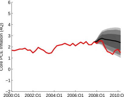
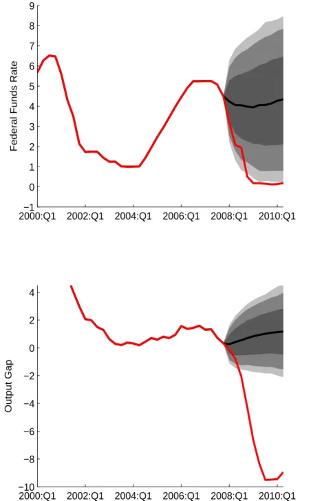
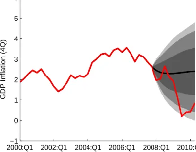
Figure 1 summarizes results from stochastic simulations of the FRB/US model for the output gap, the unemployment rate, core PCE price inflation, and the federal funds rate over the period 2008 to 2012. As can be seen, the model prior to the crisis would have viewed the subsequent evolution of real activity and short-term interest rates as extremely improbable, in that actual conditions by 2010 fall far outside the 95 percent confidence band about the late 2007 projection.9 In contrast, the model is not surprised by the behavior of inflation during the
8 In principle, we could modify the TVP-VAR and LW models so that they generate stationary steady states by imposing stationarity on all model parameters. Such an undertaking lies outside the scope of the present paper and we leave this to future research.
9 With hindsight, FRB/US sees the economy as having been hit primarily by huge shocks to the demand for new houses and to the value of residential real estate. By themselves, these shocks account for about half of the widening of the output gap seen since late 2007. In addition, shocks to risk premiums for corporate bonds, equity and the dollar account for another third of the fall in aggregate output. In contrast, EDO sees the economy as primarily having primarily been hit with a big, persistent risk-premium shock in late 2008 and during the first half of 2009. In 2008Q4, the estimated economy-wide risk premium was two standard deviations away from its mean
downturn, given the modest degree of disinflation that has occurred to date. Similar results are found in the four of the other five models; but the GARCH model is far less surprised by events. The results for the five models are shown in Figures 2 through 6.
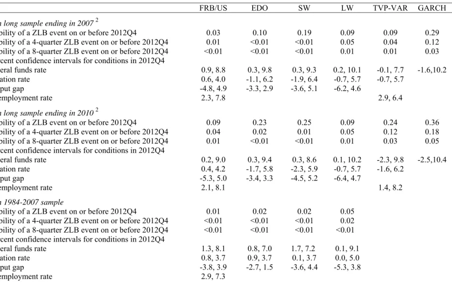
The upper panel of Table 2 reports summary statistics of the simulations used in Figures 1 through 6. The models give very different predictions regarding the probability of hitting the ZLB. The three structural models yield very small probabilities of being stuck at the ZLB for four consecutive quarters. In contrast, the three statistical models indicate that such an event would not be rare, with probabilities between 4 and 12 percent. Only the GARCH model predicts a nontrivial probability of being stuck at the ZLB for eight consecutive quarters. But even the GARCH model is surprised by the rise in the unemployment rate, as seen in Figure 6.
The bottom line of this analysis is that recent events would have been judged very unlikely prior to the crisis, based on analyses using stochastic simulations of a variety of structural and statistical models estimated on U.S. data on conditions over the past several decades. We now consider various potential sources of this underestimate of the probability of such events.
One key factor in determining the odds of hitting the ZLB is the period over which the model is estimated: Folding in the events of the past few years into the estimated variability of the economy tends to boost this probability considerably. The middle panel of table 2 reports corresponding results for simulations starting from conditions at the end of 2007 but using models where the sample period used in estimating the innovation covariance and other parameters is extended through the middle of 2010.10 Thus, these simulations take account of
the information learned over the past three years regarding both the structure of the economy and, most importantly, the incidence of large shocks during this period. Not surprisingly, the predicted probabilities of hitting the ZLB rise in most cases. More interestingly, the probabilities of being stuck at the ZLB for four or more quarters are now nontrivial in the structural models (except for SW) and sizable in the statistical models. Even so, only the TVP-VAR and GARCH models see more than a very small probability of being stuck at the ZLB for eight consecutive quarters.
under the stationary distribution; by the first half of 2009, the premium was three standard deviations away from its mean.
10 In the case of FRB/US, only the innovation covariance is reestimated using the additional data from 2008 to 2010. In the other models, all model parameters are reestimated.
Models estimated using data only from the Great Moderation period yield very small probabilities of hitting the ZLB. The lower panel of table 2 reports results from four of the models where the innovation covariances are estimated based on data from 1984-2007. Based on this sample, the three structural models see very low probabilities of hitting the ZLB and trivial probabilities of being stuck there for a year or longer. The probabilities from the LW model are higher, but only about one half as large as those based on the long sample. These results illustrate the sensitivity of quantitative analysis of the effects of the ZLB to the Great Moderation period.
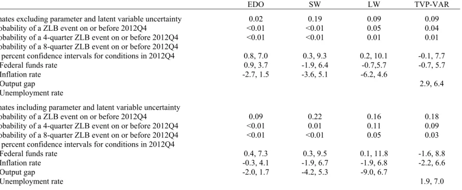
A second key factor is the incorporation of uncertainty about model parameters and latent variables in the simulations. The lower panel of table 3 reports simulation summary statistics from the four models for which we are able to adjust our estimates for uncertainty about
parameters and (in the case of LW) latent variables. In all four cases, the probabilities of hitting the ZLB rise significantly once this additional source of uncertainty is taken into account. In fact, for the two statistical models, the probability of being stuck at the ZLB for four consecutive quarters doubled, while the probability of being stuck for eight quarters rose from about 1
percent to 3 or 5 percent. These results highlight the quantitative importance of these forms of uncertainty that have heretofore been neglected in analysis of the ZLB.
IV. Has the estimated probability of hitting the ZLB changed much over time?
We address this question by using the various models to estimate how the likelihood of hitting the ZLB within the next five years would have looked at different points in the past, given assessments at the time of actual and expected economic conditions and the types of shocks that could hit the economy. Ideally, we would use real-time data and real-time versions of the models to carry out such an analysis, because after-the-fact projections based on revised data sometimes provide a misleading picture of the actual outlook at the time. Such a real-time analysis is beyond the scope of this paper, however, and so we restrict ourselves to probability assessments based on model projections and error-variance assessments constructed using the vintage of data available at the time of the writing of this paper.
Specifically, we generate the model projections and error-variance estimates using historical data through the prior quarter, for each quarter from 2000 on. In this exercise, each model is used to generate a sequence of rolling 20-quarter projections and accompanying
probability distributions centered on those projections. With the exception of FRB/US, rolling estimates of model parameters are generated using historical data through the prior quarter; FRB/US’ coefficients are instead held fixed at the estimates derived from data through 2008, because the size of the model makes repeated re-estimation infeasible. In the stochastic simulations of all the models, the rolling estimates of the shock distributions are based on an expanding sample of historical model errors.
From these rolling estimates of the probability distributions for real activity, inflation, and short-term interest rates, we compute the probability at each point in time of three different ZLB events. The first probability, shown by the red lines in Figure 7a, is the likelihood at each point in time that the nominal federal funds rate or Treasury bill rate will fall below 26 basis points at least once within the next 20 quarters. The second probability, shown by the red lines in Figure 7b, is the likelihood that short-term interest rates will be below 26 basis points for at least four consecutive quarters sometime within the next 20 quarters. The third probability, shown by the red lines in Figure 7c, is the likelihood of being stuck at the ZLB for eight
consecutive quarters. Where applicable, these rolling probabilities incorporate uncertainty about parameters and latent variables as discussed above. (The estimation sample used to generate the EDO results shown in figures 7a-c starts in 1984, whereas the estimation samples of the other models start in the 1960s.)
The results show considerable variation across time in the risk of hitting the ZLB over the medium term but roughly the same pattern across models. With one exception, all the models show the odds of a ZLB event as declining during the early 2000s, after having run at elevated levels during the sluggish recovery that followed the 2001 recession. From a low around the middle of the decade, these probability estimates then begin to climb sharply, coming near or reaching 100 percent by late 2008 and remaining elevated through the end of the sample.
To varying degrees, the estimated probabilities of hitting the ZLB for at least one quarter are influenced by the Great Moderation period. In particular, there is a tendency for the models to mark down the likelihood of encountering extremely low interest rates as their estimates of the variance of macroeconomic shocks become more and more dominated by data from the Great Moderation period. This sensitivity to Great Moderation data is perhaps greatest in the TVP-VAR model, in which the innovation variances are allowed to vary over time—an additional flexibility in model specification that makes the model more sensitive to small-sample variation.
Differences across models are more pronounced regarding the probability of being persistently stuck at the ZLB. As seen in Figure 7b, the two DSGE models (EDO and SW) show the odds of being stuck for four consecutive quarters as consistently remaining close to zero until mid-2008, whereupon they rise modestly as the model’s assessments of macroeconomic
volatility begin to incorporate the events of the crisis. In contrast, FRB/US shows the odds of being stuck at the ZLB for four quarters as rising in the early 2000s and then shooting up in 2008. The results are even in more striking for the probability of being stuck for eight consecutive quarters, shown in Figure 7c. During the decade, the DSGE models consistently saw virtually no chance of this situation ever happening. This assessment differs markedly from the profile exhibited by FRB/US, primarily because output is much more inertial in FRB/US. These results may help to explain why some researchers working with DSGE models in the past have not viewed the ZLB as a serious concern.
Results from the statistical models are broadly in line with those generated with FRB/US through late 2008, although the statistical models judge that the odds of a persistent ZLB event within the next five years have since moved noticeably lower.11 Except for the LW model, even the statistical models saw very little chance of being stuck at the ZLB for eight consecutive quarters until late 2007.
The estimated probabilities plotted in figures 7a-c reflect the effects of time-variation in both the economic outlook and estimated macroeconomic volatility. To illustrate the importance of the former factor alone, we re-run the stochastic simulations with the model parameters and variance estimates fixed at their 2010 end-of-sample values. These simulations provide a
retrospective view on the model-based probabilities of ZLB events. The results are shown by the blue lines in figures 7a-c. Consistent with the results reported in table 2, adding the data from the recent few years generally causes the model estimates of the probabilities of various ZLB events to rise. The effects of using end-of-sample parameter/variance estimates in place of rolling estimates are greatest for the probability of hitting the ZLB at least once in the next 20 quarters, and are relatively modest for the probability of being stuck at the ZLB for a year or longer.
11 Of the various model estimates of the probability of a persistent ZLB event, the ones generated by FRB/US appear to be closest to the current views of financial market participants, given that options on Eurodollar futures and interest rate caps currently indicate very low odds of the federal funds rate rising above 50 basis points before early 2012.
V. How severely did the ZLB bind during the crisis?
The evidence presented so far suggests that monetary policy may have been importantly constrained by the ZLB during the crisis, given that FRB/US and the statistical models estimate that the probability of experiencing a persistent ZLB episode in the future rose to a very high level during the crisis. By themselves, however, these statistics do not directly measure the degree to which monetary policy was constrained by the ZLB during the crisis, nor the resultant deterioration in economic performance. To address this issue, we now consider results from counterfactual simulations of FRB/US in which we explore how conditions over the last two years might have evolved had it been possible to push nominal interest rates below zero.
What monetary policy would have done in the absence of the zero lower bound constraint depends, of course, on policymakers’ judgments about how best to respond to changes in current and projected economic conditions in order to promote price stability and maximum sustainable employment. Such judgments would have depended on many factors, including assessments of overall resource utilization, the outlook for employment growth and inflation, the risks to that outlook, and the perceived responsiveness of real activity and prices to additional monetary stimulus. Because we cannot hope to account for all the factors that influence the FOMC’s decision process, we restrict ourselves to reporting results from counterfactual simulations of the FRB/US model in which the federal funds rate is allowed to follow the unconstrained
prescriptions of three different simple policy rules. Specifically, we use the standard Taylor (1993) rule, the more-aggressive rule described in Taylor (1999), and the estimated inertial rule specified previously in equation 1.5. In all three rules, the inflation target is expressed in terms of core PCE inflation and is assumed to equal 2 percent. 12
The baseline used in these counterfactual simulations matches the actual evolution of real activity and inflation through the early fall of 2010; beyond this point, we match the baseline to the extended Blue Chip consensus outlook published in October 2010. As illustrated by the black lines in the panels of figure 8, this baseline shows the economy emerging only slowly from a deep recession, accompanied by an undesirably low rate of inflation for several years and a prolonged period of near-zero short-term interest rates. Specifically, the baseline unemployment rate peaks at about 10 percent in late 2009 and then slowly drifts down over the next seven years,
12 In the economic projections published quarterly by the FOMC since early 2009, most Committee participants reported that their long-run inflation projection (as measured by the PCE price index) equaled 2 percent.
stabilizing at 6 percent towards the end of the current decade. Inflation, after bottoming out at 1 percent in late 2010, gradually drifts up as the recovery proceeds, settling in at 2 percent after 2012. And the federal funds rate remains at its effective lower bound until the second half of 2011 and then gradually returns to a more normal level of about 4 percent by the middle of the decade.13
Unfortunately, the Blue Chip survey does not provide explicit information about private forecasters’ assumptions for the supply side of the economy—a necessary input for our analysis because all three policy rules respond to movements in economic slack. However, we can infer survey participants’ estimates for the NAIRU—whether explicit or implicit—because the long-run consensus forecast shows the unemployment rate stabilizing late in the decade at 6 percent, accompanied by stable output growth and inflation.14 Using Okun’s Law, we adjust this figure to approximate the output gap implicit in the baseline by assuming thatYt
6Ut
/ 2, or approximately minus 8 percent currently. The extended Blue Chip forecast also provides information about private forecasters’ implicit estimates of the equilibrium real interest rate R* that appears in the three policy rules, in that the consensus forecast shows the real federal funds rate settling down at about 2 percent in the long run.The blue, red, and orange lines of figure 8 show simulated outcomes when the federal funds rate follows the prescriptions of the different unconstrained policy rules. Under the Taylor (1993) rule, the prescribed path of the nominal federal funds rate differs little from the baseline path, and accordingly the paths for the unemployment rate and core inflation are only slightly better (blue lines). Accordingly, a policymaker who wished to follow this rule would not have felt constrained by the ZLB, after taking account of the additional stimulus the FOMC was able to provide through the Federal Reserve’s large-scale purchases of longer-term assets. (The latter
13 Participants in the October 2010 Blue Chip survey provided forecasts of quarterly real GDP growth, the unemployment rate, overall CPI inflation, the rate on 3-month Treasury bills, and the yield on 10-year Treasury bonds through the end of 2010; in addition, participants provided annual projections for these series for the period 2011 through 2020. Because our optimal-control procedure uses the federal funds rate instead of the Treasury bill rate, we translate the projections of the latter into forecasts of the former by assuming they were equal. In the case of inflation, we translate Blue Chip forecasts for the CPI into projections for core PCE prices using the projections of the spread between these two series that were reported in the 2010Q3 Survey of Professional Forecasters. 14 This assumption is reasonably consistent with results from the 2010Q3 Survey of Professional Forecasters, in which the consensus estimate of the NAIRU was reported to be 5¾ percent. An interesting implication of these figures is that private forecasters apparently believe that the financial crisis and the accompanying deep recession have had highly persistent adverse consequences for labor market functioning, given that the Blue Chip long-run projections made prior to the crisis showed the unemployment rate stabilizing at 4¾ percent.
point is discussed in greater detail in the next section.) However, a policymaker who wished to respond more aggressively to economic slack and low inflation, and so wanted to go beyond the stimulus provided by a zero nominal funds rate and the FOMC’s asset-purchase program, would have felt constrained. Under the estimated inertial rule, for example, the counterfactual
simulation shows the nominal federal funds rate moving down to minus 1 percent by late 2009 and then remaining persistently below zero until 2012 (orange lines). As a result of this more accommodative policy, FRB/US predicts that the unemployment rate would have peaked at a somewhat lower level and would have been expected to decline considerably faster over the next few years than anticipated in the Blue Chip consensus forecast. In addition, inflation under the inertial policy rule would not have fallen as low and would be expected to run in the vicinity of 2½ percent over the next few years. As indicated by the red lines, broadly similar results for real activity and inflation are also generated under the Taylor (1999) rule, although the contour of the federal funds rate path is somewhat different. In particular, the Taylor (1999) rule calls for a steeper decline in nominal short-term interest rates in 2009 but a somewhat faster
renormalization of monetary policy starting in 2011.
Figure 9 also presents simulation results when the counterfactual path of the federal funds rate is set “optimally”, as defined using optimal-control techniques to find that the unconstrained path of short-term interest rates that would minimize a policymaker loss function. Here we modify an approach regularly used in by Federal Reserve staff in FOMC-related analyses—see Svensson and Tetlow (2005)—to compute what path of the unconstrained nominal funds rate from 2009Q1 on would have minimized deviations of resource utilization from zero and inflation from 2 percent, subject to the baseline economic outlook and the dynamics of the FRB/US model. The specific loss function used in our analysis is:
(1.8)
2
2 20
.99 6 2
m j
t t j t j t j
j
L E U R
,where U denotes the unemployment rate; π denotes inflation, measured by the four-quarter percentage change in the chain-weighted core PCE price index; and R denotes the nominal funds rate. As can be seen, this specification penalizes large quarter-to-quarter changes in the nominal funds rate in addition to deviations of U from the NAIRU and π from the 2 percent inflation
target; the third term serves to damp excessively sharp movements in the funds rate that might otherwise occur.15
As indicated by the green line in figure 8, “optimal” policy in the absence of the ZLB constraint would have called for pushing the federal funds rate more than 400 basis points below zero by mid 2010, and then keeping short-term interest rates persistently below zero until early 2013. Based on the dynamics of the FRB/US model under rational expectations, such a policy would have induced a sharp drop in long-term interest rates in early 2009 that would have stimulated real activity directly through cost-of-capital effects as well as indirectly through higher wealth and a lower real foreign exchange value of the dollar. As result, the
unemployment rate would have peaked at only 9 percent and would have fallen back to a more normal level much more quickly than currently anticipated by private forecasters. Moreover, agents—recognizing the more favorable longer-run prospects for the real economy under this monetary policy—would have raised their expectations for inflation in the medium term, which in turn would have helped to support actual inflation in the short run. As a result, FRB/US predicts that inflation would have fluctuated at a level modestly above the 2 percent target for a time.
On balance, these counterfactual simulation results suggest that the severity of the ZLB constraint has been considerable over the past few years. Indeed, under some assumptions, a policymaker could have arguably wished to push the nominal funds rate several hundred basis points below zero. These results are consistent with those of Williams (2009). That said, we should note several caveats to this conclusion.
First, our results are conditioned on the dynamics of the FRB/US model, and other models might yield different results. Indeed, exploratory optimal-control simulations carried out with the EDO and the SW models suggest that these models would have called for a less
dramatic easing in unconstrained optimal monetary policy than FRB/US. The source of this difference between FRB/US and these models appears to be a greater sensitivity of real activity and inflation in the DSGE models to anticipated monetary policy shocks—a property that in turn
15 In solving the optimal-control problem, we set the length of the evaluation window, m, at 100 quarters but only minimize the function with respect to the values of R over the first 60 quarters; beyond that point, the funds rate is assumed to follow the path prescribed by the estimated policy rule embedded in the three models. These settings are sufficient to ensure that the simulated path of the funds rate follows an essentially flat trajectory at the end of the 60-quarter optimization window and beyond.
reflects a higher relative degree of intrinsic persistence in FRB/US. Reflecting this greater sensitivity to anticipated policy actions, the DSGE models see much more scope for
policymakers to mitigate the effects of the ZLB by promising to run an easier monetary policy in the future, when the ZLB constraint no longer binds. Even assuming that this aspect of the dynamics of the DSGE models is empirically valid, the actual effectiveness of such promissory policies for mitigating the effects of the ZLB would depend critically on the ability of
policymakers to credibly commit to future policy actions.
Second, the FRB/US simulation results may overstate the severity of the ZLB constraint during the current downturn because of our flaws in the baseline supply-side assumptions. As noted above, we calibrated the NAIRU in the baseline to the long-run Blue Chip projections of the unemployment rate, implying a current output gap of roughly minus 8 percent. However, estimates of the output gap reported by official institutions such as the IMF (2010), the OECD (2010), and the Congressional Budget Office (2010) are somewhat smaller, ranging from minus 5.1 percent to minus 7.2 percent; some estimates reported by Weidner and Williams (2009) indicate even less slack. Using these less-pronounced estimates of slack in place of the baseline assumption would noticeably shrink the estimated severity of the ZLB constraint under all the various monetary policy assumptions.
Third, the dynamics of the FRB/US model may not provide an accurate characterization of the likely responses of real activity and inflation to changes in the federal funds rate in current circumstances. For example, the interest-sensitivity of aggregate demand may now be unusually low because of reduced access to credit or heightened uncertainty about the economic outlook. If so, an unconstrained optimal policy response might conceivably call for a larger peak decline in the nominal funds rate.
Finally, we should stress that the loss function used in the optimal-control analysis is only illustrative, and may not accurately characterize policymakers’ preferences. For example,
policymakers may implicitly score the loss from a percentage point increase in the
unemployment gap as different from that associated with a percentage point increase in the inflation gap, instead of weighing them as equal as the loss function assumes. Moreover, the quadratic loss function abstracts from any special concerns that policymakers might have about extreme tail risks. Such risks are of particular concern in current circumstances, given the
asymmetries in probabilities created by the zero lower bound and the resultant increase in the likelihood of deflation.
VI. Did large-scale asset purchases significantly ease the ZLB constraint?
On balance, we judge the results presented in the previous section as indicating that conventional monetary policy in the United States has been importantly constrained by the ZLB recently, in that a variety of counterfactual simulations using various policy rules would have called for pushing the nominal federal funds rate well below zero if that had been possible. An important aspect of recent monetary policy sidestepped in those simulations was the role of the Federal Reserve’s purchases of longer-term Treasury securities and agency debt and mortgage-backed securities (MBS). To the degree that these purchases have mitigated the depth and duration of the recession and improved the prospects for economic recovery, they provided monetary stimulus beyond what was possible through conventional means. Alternatively put, if the Federal Reserve had not taken these actions, the counterfactual simulations would
presumably have shown the federal funds rate moving even further into negative territory, because the policy prescriptions would have been conditioned on even worse outcomes for unemployment and inflation in 2009 and 2010, and an even less favorable outlook for 2011 and beyond.16
A primary objective of large-scale asset purchases is to put additional downward pressure on longer-term yields at a time when short-term interest rates have already fallen to their
effective lower bound. Because of spillover effects on other financial markets, such a reduction in longer-term yields should lead to more accommodative financial conditions overall, thereby helping to stimulate real activity and to check undesirable disinflationary pressures through a variety of channels, including reduced borrowing costs, higher stock valuations, and a lower foreign exchange value of the dollar. In many ways, this transmission mechanism is similar to the standard one involved in conventional monetary policy, which primarily operates through the
16 In addition to large-scale asset purchases, the Federal Reserve also implemented a number of emergency credit and liquidity programs with the objective of improving market functioning and mitigating contagion effects at a time of extreme stress in many financial markets. (See www.federalreserve.gov/newsevents/reform_transaction.htm for further details.) These programs played an important role in keeping the financial crisis and the recession from becoming even deeper and more prolonged. However, our models lack the extremely detailed financial linkages required to quantify the macroeconomic impact of these programs, and so we do not analyze their effects in this paper.
influence on long-term yields of changes to the current and expected future path of the federal funds rate.
Because of this similarity, we can use our structural models to obtain a rough estimate of the macroeconomic effects of large-scale asset purchases, specifically by combining the FRB/US model with a simple model of the influence of Federal Reserve holdings of longer-term assets on the term premium embedded in long-term yields. Ideally, we would carry out a similar analysis using the EDO and Smets-Wouters models but the structure of those particular DSGE models unfortunately does not lend itself to such an exercise.17 However, other DSGE models, such as the one developed by Andres, Lopez-Salido, and Nelson (2004) that incorporates imperfect substitution among assets into the standard new Keynesian framework, could be used for this type of analysis.
One way to view the effects of asset purchases on long-term interest rates is through their implications for the price demanded by market participants to expose themselves to some of the risks involved in lending long-term. In the case of Treasury securities, these risks primarily center on the uncertain path for future inflation and help to explain why the yield curve generally slopes up: Risk-averse investors do not like to assume this risk and so require a compensating term premium for holding longer-term Treasury securities in place of Treasury bills—a premium that might rise if the government or the central bank were to increase the average duration of government debt supplied to the market. Term premiums can also be viewed as arising from the existence of preferred-habit investors whose willingness to buy securities of a given maturity is an increasing function of the yield on that asset; Vayanos and Vila (2009) have incorporated such investors into a no-arbitrage model in which yields on securities of different maturities are linked in a manner that depends in part on their relative supplies. An implication of such
preferred-habit effects is that the central bank should be able to lower long-term interest rates if it can substantially reduce the stock of long-term debt held by the private sector.
To accomplish such a reduction, the Federal Reserve purchased about $1.25 trillion in agency MBS, $170 billion in agency debt, and $300 billion in longer-term Treasury securities
17 In FRB/US, bond yields that embed term premiums play a direct role in influencing real activity through the cost of capital; long-term interest rates also influence real activity indirectly through the stock market and the exchange rate. In contrast, real activity in EDO and Smets-Wouters depends on expectations for the future path of short-term interest rates, not on actual long-term asset prices, and so term premium shocks do not enter the models. As documented by Rudebusch, Sack and Swanson (2007), however, econometric evidence suggests that a reduction in term premiums implies stronger future real activity, independent of other interest rate effects.
over the course of 2009 and early 2010, with the purchases reflected in an increase in banks’ reserve balances held at the Federal Reserve Banks. More recently, the FOMC announced at its November 2010 meeting that it intends to purchase another $600 billion in longer-term Treasury securities by the middle of 2011; in addition, the FOMC stated its intention to continue
reinvesting principal payments on its asset holdings in Treasury notes and bonds, a policy first announced at the August 2010 meeting. Because of these actions, and taking account of earlier redemptions and MBS principal payments, security holdings in the Federal Reserve’s System Open Market Account (SOMA) are expected to climb to $2.6 trillion by the middle of 2011, with essentially all of these assets having an original maturity of greater than one year. In contrast, SOMA security holdings prior to the crisis in mid-2007 were only $790 billion, $280 billion of which were in Treasury bills (that is, securities with original maturities of less than one year).
Several recent studies have attempted to estimate the quantitative effect of large-scale asset purchases by the Federal Reserve on U.S. long-term interest rates, including Gagnon et al. (2010), D’Amico and King (2010), Doh (2010), Hamilton and Wu (2010), and Swanson (2010). Other researchers have examined the quantitative effects of similar unconventional policy
actions recently carried out abroad, such as the Bank of England’s quantitative-easing program; see Meier (2009) and Joyce et al. (2010). In the case of the U.S. studies, researchers have employed a variety of techniques, including:
event studies of movements in yields following major FOMC announcements about asset
purchases in late 2008 and 2009 (Gagnon et al.),18
time-series regressions using reduced-form models of long-term interest rates that include variables to capture the effects of recent changes in SOMA asset holdings (Gagnon et al., Doh),
and a version of the formal model of the term structure proposed by Vayanos and Vila, estimated using pre-crisis data from 1990 to 2007 and adapted to predict how long-term yields should respond to large-scale asset purchases when short-term interest rates are at the zero lower bound (Hamilton and Wu).
18 Swanson (2010) uses an event study to reexamine the effects of “Operation Twist”, the attempt by the U.S. government in 1961 to lower long-term yields by altering the relative supplies of longer-term and short-term Treasury debt. He concludes that the program lowered long-term yields by about 15 basis points—a finding that, after adjusting for scale, is in line with the effects reported by Gagnon et al. for the Federal Reserve’s 2009 program.
Although these studies yield a range of estimates for the effects of the original 2009 asset
purchase program, the general conclusion seems to be that this first phase of the expansion of the Federal Reserve’s asset holdings significantly reduced the general level of long-term interest rates. In particular, these studies suggest on balance that the Federal Reserve’s 2009 purchases probably lowered the yield on the 10-year Treasury note as well as high-grade corporate bonds by around 50 basis points.19 That said, considerable uncertainty attends this estimate; for
example, the estimates reported in Gagnon et al. range from a low of 30 basis points to a high of 100 basis points.
One way to put this effect on long-term yields in 2009 into perspective is to translate it into an equivalent cut in the federal funds rate. Regressing quarterly changes in the 10-year Treasury yield on quarterly changes in the federal funds rate for the period 1987 through 2007 yields a coefficient of about 0.25, implying that a 100 basis point reduction in short-term interest rates is typically associated with a 25 basis point decline in long-term yields. Accordingly, achieving a 50 basis point drop in bond yields through conventional means rather than asset purchases should ordinarily require something like a 200 basis point cut in the federal funds rate. Based on this back-of-the-envelope calculation, the original phase of the asset purchase program arguably allowed the FOMC to supply about the same amount of additional stimulus as it could have achieved if it had been possible to push nominal short-term interest rates 200 basis points below zero.
Asset purchases could also provide important economic benefits through an improvement in market functioning. Indeed, this seems to have been the case with housing finance. Spreads of residential mortgage rates over 10-year Treasury yields, which were quite elevated by historical standards in late 2008, fell markedly over the next few months in the wake of Federal Reserve announcements about its MBS purchase program, in part because the program assured a steady demand for these securities at a time of strained market conditions. After taking account of other factors contributing to the decline in spreads, Gagnon et al. estimate that the MBS purchase program probably lowered the spread of mortgage rates over Treasury yields by about 50 basis points. However, this effect was probably temporary because, even in the absence of
19 Estimates reported in Meier (2009) and Joyce et al (2010) for the effects of the Bank of England’s quantitative easing program are somewhat larger at around 100 basis points.
action by the Federal Reserve, spreads would have presumably come down eventually as the financial crisis passed and the economy began to recover.
Finally, the Federal Reserve’s asset purchase program could potentially have stimulated real activity by changing public perceptions about the likely longer stance of monetary policy, conventional and unconventional; for example, it may have led market participants to expect that the FOMC would respond more aggressively to high unemployment and undesirably low
inflation than was previously thought. In a similar vein, initiation of the program may have diminished public perceptions of the likelihood of extreme tail events, such as deflation, potentially lowering risk premiums and increasing household and business confidence, thereby raising agents’ willingness to spend.
For a more complete assessment of the possible macroeconomic benefits of the Federal Reserve’s elevated asset holdings, including the effects of the recently announced $600 billion expansion of the program, we now turn to simulations of the FRB/US model. For this exercise, we need to go beyond the initial impact of the original asset purchase program and specify how the evolution of SOMA holdings of longer-term securities influences term premiums over time. To do this, we specify a simple model of portfolio-balance effects, described in appendix A1. In this model, the size of the term premium effect at any point in time is assumed to be proportional to the discounted present value of expected future SOMA holdings of longer-term securities in excess of what the Federal Reserve would normally hold, relative to the level of nominal GDP. An implication of this model is that the magnitude of the term-premium effect depends not just on the amount of longer-term assets currently held by the Federal Reserve but also on investors’ expectations for the evolution of these holdings over time.20 Although the model is somewhat ad hoc, we note that it mimics the behavior of the more elaborate term-structure model estimated by Hamilton and Wu.
Figure 9 summarizes the predictions of this simple model for the evolution of portfolio-balance effects arising from the Federal Reserve’s large-scale asset purchases. Under the first phase of the program, which effectively began in early 2009 and is assumed to have lasted into
20 Such forward-looking behavior is consistent with the response of market interest rates to the original 2009 program, in that yields moved sharply in response to announcements about future purchases that would not be completed for many months. Similar behavior was observed again between late August 2010 and the November 2010 FOMC meeting, when market participants gradually came to anticipate a second round of asset purchases—an anticipation that led to noticeable decline in long-term yields in advance of the actual FOMC announcement.