Detecting Large-Scale System Problems by Mining Console Logs
Wei Xu
∗Ling Huang
†Armando Fox
∗David Patterson
∗Michael I. Jordan
∗∗EECS Department
University of California at Berkeley, USA
{xuw,fox,pattrsn,jordan}@cs.berkeley.edu
†Intel Labs Berkeley
Berkeley, CA, USA [email protected]
Abstract
Surprisingly, console logs rarely help operators detect problems in large-scale datacenter services, for they of-ten consist of the voluminous intermixing of messages from many software components written by independent developers. We propose a general methodology to mine this rich source of information to automatically detect system runtime problems. We first parse console logs by combining source code analysis with information re-trieval to create composite features. We then analyze these features using machine learning to detect opera-tional problems. We show that our method enables analy-ses that are impossible with previous methods because of its superior ability to create sophisticated features. We also show how to distill the results of our analysis to an operator-friendly one-page decision tree showing the critical messages associated with the detected problems. We validate our approach using the Darkstar online game server and the Hadoop File System, where we detect nu-merous real problems with high accuracy and few false positives. In the Hadoop case, we are able to analyze 24 million lines of console logs in 3 minutes. Our method-ology works on textual console logs of any size and re-quires no changes to the service software, no human in-put, and no knowledge of the software’s internals.
1
Introduction
When a datacenter-scale service consisting of hundreds of software components running on thousands of com-puters misbehaves, developer-operators need every tool at their disposal to troubleshoot and diagnose operational problems. Ironically, there is one source of information that is built into almost every piece of software that pro-vides detailed information that reflects the original de-velopers’ ideas about noteworthy or unusual events, but is typically ignored: the humble console log.
Since the dawn of programming, developers have used everything from printf to complex logging and moni-toring libraries [8, 9] to record program variable val-ues, trace execution, report runtime statistics, and even print out full-sentence messages designed to be read by a human—usually by the developer herself. However,
modern large-scale services usually combine large open-source components authored by hundreds of develop-ers, and the people scouring the logs—part integrator, part developer, part operator, and charged with fixing the problem—are usually not the people who chose what to log or why. (We’ll use the term operator to represent a potentially diverse set of people trying to detect opera-tional problems.) Furthermore, even in well-tested code, many operational problems are dependent on the deploy-ment and runtime environdeploy-ment and cannot be easily re-produced by the developer. To make things worse, mod-ern systems integrate extmod-ernal (often open source) com-ponents that are frequently revised or upgraded, which may change what’s in the logs or the relevance of certain messages. Keeping up with this churn rate exacerbates the operators’ dilemma. Our goal is to provide them with better tools to extract value from the console logs.
As logs are too large to examine manually [14, 22] and too unstructured to analyze automatically, operators typi-cally create ad hoc scripts to search for keywords such as “error” or “critical,” but this has been shown to be insuffi-cient for determining problems [14, 22]. Rule-based pro-cessing [24] is an improvement, but the operators’ lack of detailed knowledge about specific components and their interactions makes it difficult to write rules that pick out the most relevant sets of events for problem detection. Instead of asking users to search, we provide tools to au-tomatically find “interesting” log messages.
Since unusual log messages often indicate the source of the problem, it is natural to formalize log analysis as an anomaly detection problem in machine learning. How-ever, it is not always the case that the presence, absence or frequency of a single type of message is sufficient to pinpoint the problem; more often, a problem manifests as an abnormality in the relationships among different types of log messages (correlations, relative frequencies, and so on). Therefore, instead of analyzing the words in textual logs (as done, for example, in [27]), we cre-ate features that accurcre-ately capture various correlations among log messages, and perform anomaly detection on these features. Creating these features requires augment-ing log parsaugment-ing with information about source code; our
method for doing this augmentation is part of our contri-bution.
We studied logs and source code of many popular soft-ware systems used in Internet services, and observed that a typical console log is much more structured than it ap-pears: the definition of its “schema” is implicit in the log printing statements, which can be recovered from pro-gram source code. This observation is key to our log parsing approach, which yields detailed and accurate fea-tures. Given the ubiquitous presence of open-source soft-ware in many Internet systems, we believe the need for source code is not a practical drawback to our approach.
Our contribution is a general four-step methodology that allows machine learning and information retrieval techniques to be applied to free-text logs to find the “needles in the haystack” that might indicate operational problems, without any manual input. Specifically, our methodology involves the following four contributions:
1) A technique for analyzing source code to recover the structure inherent in console logs;
2) The identification of common information in logs— state variables and object identifiers—and the automatic creation of features from the logs (exploiting the struc-ture found) that can be subjected to analysis by a variety of machine learning algorithms;
3) Demonstration of a machine learning and informa-tion retrieval methodology that effectively detects un-usual patterns or anomalies across large collections of such features extracted from a console log;
4) Where appropriate, automatic construction of a vi-sualization that distills the results of anomaly detection in a compact and operator-friendly format that assumes no understanding of the details of the algorithms used to analyze the features.
The combination of elements in our approach, in-cluding our novel combination of source code analysis with log analysis and automatic creation of features for anomaly detection, enables a level of detail in log analy-sis that was previously impossible due to the inability of previous methods to correctly identify the features nec-essary for problem identification.
Our approach requires no changes to existing soft-ware and works on existing textual console logs of any size, and some of the more computationally expensive steps are embarrassingly parallel, allowing us to run them as Hadoop [2] map-reduce jobs using cloud computing, achieving nearly linear speedup for a few dollars per run. We evaluate our approach and demonstrate its capa-bility and scalacapa-bility with two real-world systems: the Darkstar online game server [28] and the Hadoop File System. For Darkstar, our method accurately detects per-formance anomalies immediately after they happen and provides hints as to the root cause. For Hadoop, we de-tect runtime anomalies that are commonly overlooked,
starting: xact 325 is COMMITTING starting: xact 346 is ABORTING
1 CLog.info("starting: " + txn); 2 Class Transaction {
3 public String toString() { 4 return "xact " + this.tid + 5 " is " + this.state;
6 }
7 }
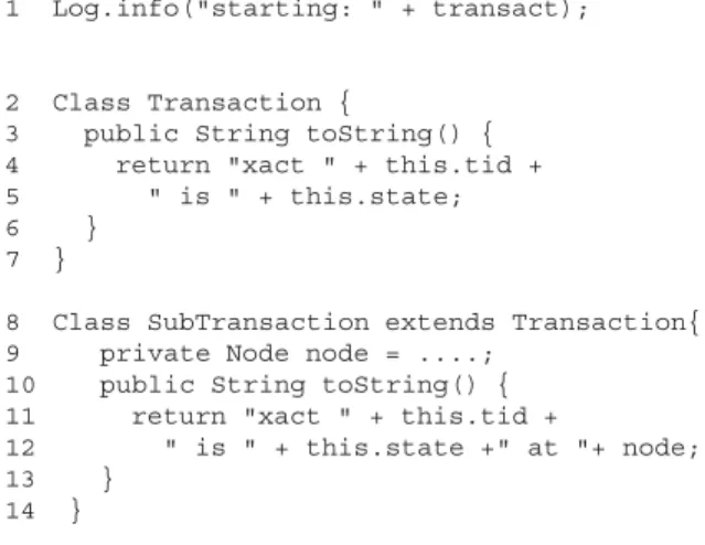
Figure 1: Top: two lines from a simple console log. Bot-tom: Java code that could produce these lines.
and distill over 24 million lines of console logs (col-lected from 203 Hadoop nodes) to a one-page decision tree that a domain expert can readily understand. This automated process can be done with Hadoop map-reduce on 60 Amazon EC2 nodes within 3 minutes.
Section 2 provides an overview of our approach, tion 3 describes our log parsing technique in detail, Sec-tions 4 and 5 present our soluSec-tions for feature creation and anomaly detection, Section 6 evaluates our approach and discusses the visualization technique, Section 7 dis-cusses extensions and provide suggestions to improve log quality, Section 8 summarizes related work, and Sec-tion 9 draws some conclusions.
2
Overview of Approach
2.1 Information buried in textual logs
Important information is buried in the millions of lines of free-text console logs. To analyze logs automatically, we need to create high quality features, the numerical representation of log information that is understandable by a machine learning algorithm. The following three key observations lead to our solution to this problem. Source code is the “schema” of logs. Although con-sole logs appear in free text form, they are in fact quite structured because they are generated entirely from a rel-atively small set of log printing statements in the system. Consider the simple console log excerpt and the source code that generated it in Figure 1. Intuitively, it is easier to recover the log’s hidden “schema” using the source code information (especially for a machine). Our method leverages source code analysis to recover the in-herit structure of logs. The most significant advantage
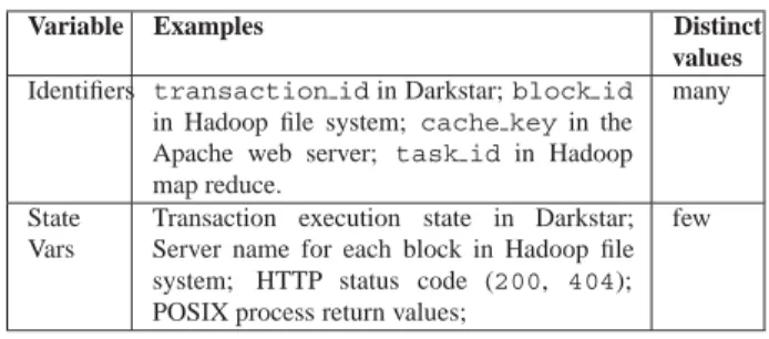
Variable Examples Distinct values
Identifiers transaction idin Darkstar;block id in Hadoop file system; cache keyin the Apache web server; task id in Hadoop map reduce.
many
State Vars
Transaction execution state in Darkstar; Server name for each block in Hadoop file system; HTTP status code (200, 404); POSIX process return values;
few
starting: xact 325 is PREPARING prepare: xact 325 is COMMITTING comitted: xact 325 is COMMITTED
1. Log Parsing
type=1, tid=325, state=PREPARING type=2, tid=325, state= COMMITTING
type=3, tid=325, state=COMMITTED 1 1 1 0 0 0 0 0 0
1 0 1 0 0 0 0 0 0 1 1 1 0 1 0 0 0 0
2. Feature creation 3. Anomaly
detection 4.Visualization
Message Count Vectors State Ratio Vector
PREPARING
COMMITTING COMMITTED
ABORTED
PCA Anomaly Detection
325: 326: 327: Source Code
Raw Console Log Structured Log
starting: xact (.*) is (.*)
Message template
void startTransaction(){ …
LOG.info(“starting” + transact); }
Decision Tree
At time window 100
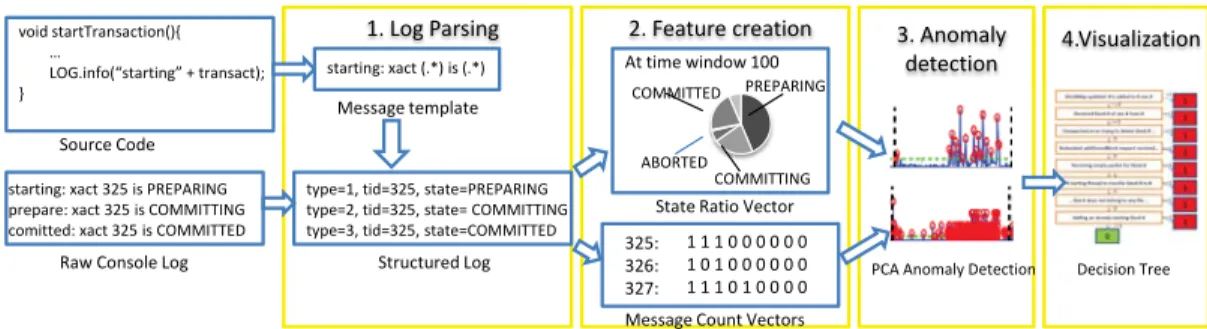
Figure 2:Overview of console log analysis work flow.
of our approach is that we are able to accurately parse all possible log messages, even the ones rarely seen in actual logs. In addition, we are able to eliminate most heuristics and guesses for log parsing used by existing solutions. Common log structures lead to useful features. A person usually reads the log messages in Figure 1 as a constant part (starting: xact... is) and multiple variable parts (325/326 and COMMITTING/ABORTING). In this paper, we call the constant part the message type and the variable part the message variable.
Message types—marked by constant strings in a log message—are essential for analyzing console logs and have been widely used in earlier work [17]. In our anal-ysis, we use the constant strings solely as markers for the message types, completely ignoring their semantics as English words, which is known to be ambiguous [22]. Message variables carry crucial information as well. In contrast to prior work that focuses on numerical vari-ables [17, 22, 35], we identified two important types of message variables for problem detection by studying logs from many systems and by interviewing Internet service developers/operators who heavily use console logs. We acknowledge that logs also contain other types of mes-sage variables such as timestamps and various counts. We do not discuss those variables in this paper as they have been well studied in existing work [27].
Identifiers are variables used to identify an object ma-nipulated by the program (e.g., the transaction ids325
and346in Figure 1), while state variables are labels that enumerate a set of possible states an object could have in program (e.g.COMMITTINGandABORTINGin Figure 1). Table 1 provides extra examples of such variables. We can determine whether a given variable is an identifier or a state variable progmatically based on its frequency in console logs. Intuitively, state variables have a small number of distinct values while identifiers take a large number of distinct values (detailed in Section 4).
Message types and variables contain important run-time information useful to the operators. However, lack-ing tools to extract these structures, operators either ig-nore them, or spend hours greping and manually exam-ining log messages, which is tedious and inefficient.
Our accurate log parsing allows us to use structured
information such as message types and variables to au-tomatically create features that capture information con-veyed in logs. To our knowledge, this is the first work ex-tracting information at this fine level of granularity from console logs for problem detection.
Messages are strongly correlated. When log messages are grouped properly, there is a strong and stable corre-lation among messages within the same group. For ex-ample, messages containing a certain file name are likely to be highly correlated because they are likely to come from logically related execution steps in the program.
A group of related messages is often a better indi-cator of problems than individual messages. Many anomalies are only indicated by incomplete message se-quences. For example, if a write operation to a file fails silently (perhaps because the developers do not handle the error correctly), no single error message is likely to indicate the failure. By correlating messages about the same file, however, we can detect such cases by observ-ing that the expected “closobserv-ing file” message is missobserv-ing. Previous work grouped logs by time windows only, and the detection accuracy suffers from noise in the correla-tion [14, 27, 35]. In contrast, we create message groups based on more accurate information, such as the message variables described above. In this way, the correlation is much stronger and more readily encoded so that the ab-normal correlations also become easier to detect. 2.2 Workflow of our approach
Figure 2 shows the four steps in our general framework for mining console logs.
1) Log parsing. We first convert a log message from unstructured text to a data structure that shows the mes-sage type and a list of mesmes-sage variables in (name, value) pairs. We get all possible log message template strings from the source code and match these templates to each log message to recover its structure (that is, message type and variables). Our experiments show that we can achieve high parsing accuracy in real-world systems.
There are systems that use structured tracing only, such as BerkeleyDB (Java edition). In this case, because logs are already structured, we can skip this first step and directly apply our feature creation and anomaly
detec-System Lang Logger Msg Construction LOC LOL Vars Parse ID ST Operating system
Linux (Ubuntu) C custom printk + printf wrap 7477k 70817 70506 Y Yb Y
Low level Linux services
Bootp C custom printf wrap 11k 322 220 Y N N
DHCP server C custom printf wrap 23k 540 491 Y Yb Y
DHCP client C custom printf wrap 5k 239 205 Y Yb Y
ftpd C custom printf wrap 3k 66 67 Y Y N
openssh C custom printf wrap 124k 3341 3290 Y Y Y
crond C printf printf wrap 7k 112 131 Y N Y
Kerboros 5 C custom printf wrap 44k 6261 4971 Y Y Y
iptables C custom printf wrap 52k 2341 1528 Y N Y
Samba 3 C custom printf wrap 566k 8461 6843 Y Y Y
Internet service building blocks
Apache2 C custom printf wrap 312k 4008 2835 Y Y Y
mysql C custom printf wrap 714k 5092 5656 Y Yb Yb
postgresql C custom printf wrap 740k 12389 7135 Y Yb Yb
Squid C custom printf wrap 148k 2675 2740 Y Y Y
Jetty Java log4j string concatenation 138k 699 667 Y Y Y
Lucene Java custom custom log function 217k 143 159 Ya Y N
BDB (Java) Java custom custom structured trace 260k - - - Y N
Distributed systems
Hadoop Java custom log4j string concatenation 173k 911 1300 Y Y Y
Darkstar Java jdk-log Java format string 90k 578 658 Y Yb Yb
Nutch Java log4j string concatenation 64k 507 504 Y Y Y
Cassandra Java log4j string concatenation 46k 393 437 Y N Y
Storage Prototype C custom custom structured trace -c -c -c -c Y Y
aLogger class is not consistent in every module, so we need to manually specify the logger function name for each module. bSystem prints minimal amount of logs by default, so we need to enable debug logging.
cSource code not available, but logs are well structured so manual parsing is easy.
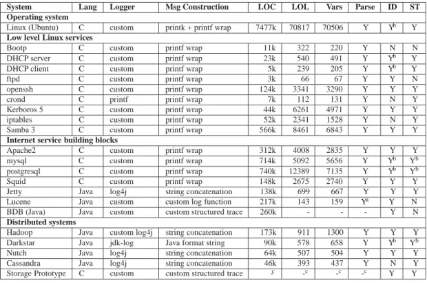
Table 2: Console logging in popular software systems. LOC = lines of codes in the system. LOL = number of log printing statements. Vars = number of variables reported in log messages. Parse = whether our source analysis based parsing applies. ID = whether identifier variables are reported. ST = whether state variables are reported.
tion methods. Note that these structured logs still contain both identifiers and state variables.1
2) Feature creation. Next, we construct feature vectors from the extracted information by choosing appropriate variables and grouping related messages. In this paper, we focus on constructing the state ratio vector and the message count vector features, which are unexploited in prior work. In our experiments with two large-scale real-world systems, both features yield good detection results. 3) Anomaly detection. Then, we apply anomaly de-tection methods to mine feature vectors, labeling each feature vector as normal or abnormal. We find that the Principal Component Analysis (PCA)-based anomaly detection method [5] works very well with both features. This method is an unsupervised learning algorithm, in which all parameters can be either chosen automatically or tuned easily, eliminating the need for prior input from the operators. Although we use this specific machine learning algorithm for our case studies, it is not intrinsic 1In fact, the last system in Table 2 (Storage Prototype) is an anony-mous research prototype with built-in customized structured traces. Without any context, even without knowing the functionality of the sys-tem, our feature creation and anomaly detection algorithm successfully discovered log segments that the developer found insightful.
to our approach, and different algorithms utilizing differ-ent extracted features could be readily “plugged in” to our framework.
4) Visualization. Finally, in order to let system integra-tors and operaintegra-tors better understand the PCA anomaly detection results, we visualize results in a decision tree [34]. Compared to the PCA-based detector, the deci-sion tree provides a more detailed explanation of how the problems are detected, in a form that resembles the event processing rules [10] with which system integrators and operators are familiar.
2.3 Case study and data collection
We studied source code and logs from 22 widely de-ployed open source systems. Table 2 summarizes the results. Although these systems are distinct in nature, developed in different languages by different developers at different times, 20 of the 22 systems use free text logs, and our source-code-analysis based log parsing applies to all of the 20. Interestingly, we found that about 1%-5% of code lines are logging calls in most of the systems, but most of these calls are rarely, if ever, executed be-cause they represent erroneous execution paths. It is al-most impossible to maintain log-parsing rules manually
System Nodes Messages Log Size Darkstar 1 1,640,985 266 MB Hadoop (HDFS) 203 24,396,061 2412 MB Table 3: Data sets used in evaluation. Nodes=Number of nodes in the experiments.
with such a large number of distinct logger calls, which highlights our advantage of discovering message types automatically from source code. On average, a message reports a single variable. However, there are many mes-sages, such asstarting serverthat reports no vari-ables, while other messages can report 10 or more.
Most C programs use printf style format strings for logging, although a large portion uses wrapper functions to generate standard information such as time stamps and severity levels. These wrappers, even if customized, can be detected automatically from the format string pa-rameter. In contrast, Java programs usually use string concatenation to generate log messages and often rely on standard logger packages (such as log4j). Analyz-ing these loggAnalyz-ing calls requires understandAnalyz-ing data types, which we detail in Section 3. Our source-code-analysis based log parsing approach successfully works on most of them, and can find at least one of state variables and identifiers in 21 of the 22 systems in Table 2 (16 have both), confirming our assumption of their prevalence.
To be succinct yet reveal important issues in console log mining, we focus further discussion on two repre-sentative systems shown in Table 2: the Darkstar online game server and the Hadoop File System (HDFS). Both systems handle persistence, an important yet complicated function in large-scale Internet services. However, these two systems are different in nature. Darkstar focuses on small, time sensitive transactions, while HDFS is a file system designed for storing large files and batch process-ing. They represent two major open source contributors (Sun and Apache, respectively) with different coding and logging styles.
We collected logs from systems running on Amazon’s Elastic Compute Cloud (EC2) and we also used EC2 to analyze these logs. Table 3 summarizes the log data sets we used. The Darkstar example revealed a behav-ior that strongly depended on the deployment environ-ment, which led to problems when migrating from tra-ditional server farms to clouds. In particular, we found that Darkstar did not gracefully handle performance vari-ations that are common in the cloud-computing environ-ment. By analyzing console logs, we found the reason for this problem, as discussed in detail in Section 6.2.
Satisfied with Darkstar results, to further evaluate our method we analyzed HDFS logs, which are much more complex. We collected HDFS logs from a Hadoop clus-ter running on over 200 EC2 nodes, yielding 24 million lines of logs. We successfully extracted log segments
in-dicating run-time performance problems that have been confirmed by Hadoop developers.
All log data are collected from unmodified off-the-shelf systems. Console logs are written directly to local disks on each node and collected offline by simply copy-ing log files, which shows the convenience (no instru-mentation or configuration) of our log mining approach. In the HDFS experiment, we used the default logging level, while in the Darkstar experiment, we turned on de-bug logging (FINERlevel in the logging framework).
3
Log Parsing with Source Code
In addition to standard “fields” in console logs, such as timestamps, we focus on the free text part of a log message. For the log excerpt at the top of Figure 1, human readers would reasonably conclude that 325,
346, COMMITTING and ABORTING are message vari-ables while the rest are constant strings marking message types. They could then write a regular expression such as
starting: xact (.*) is (.*)to “templatize” such log messages. We want to automate the process. The difficulty. Unless the log itself is marked with formatting to distinguish these elements, we must “templatize” automatically. As discussed in Sec-tion 2.1, it is much easier for a machine to use the source code as the “schema” for console logs. If the software is written in a language like C, it is likely that the template can be directly inferred from printf variants that generate the messages, such as fprintf(LOG, "starting: xact %d is %s"), with the various escapes (%d, %f, and so on) telling us something about the types of the variables. However, it is more challenging in object-oriented (OO) languages such as Java, which are increasingly used for open source software (Table 2). Consider the excerpt of Java source shown in the bottom half of Figure 1, which generated the two example log lines. Clearly, thetidvariable of the
txnobject corresponds to the identifiers 325 and 346 in the log message of Figure 1, and thestatevariable cor-responds to the labelsCOMMITTINGandABORTING. Try-ing to extract a regular expression by simply “greppTry-ing” the source code would only give usstarting: (. *)
(line 1), which does not distinguishtidandstateas separate features with distinct ranges of possible values. Critically, as we will show later, we need this finer level of feature resolution to find “interesting” problems.
Three reasons cause this difficulty to arise in OO lan-guages. First, we need to know thatCLogidentifies a log-ger object; that is, knowing the name of the loglog-ger class is not enough. Second, the OO idiom for printing is for an object to implement atoString() method that re-turns a printable representation of itself for interpolation into a string; in this example, thetoString() method of the abstract typeTransaction actually reveals the
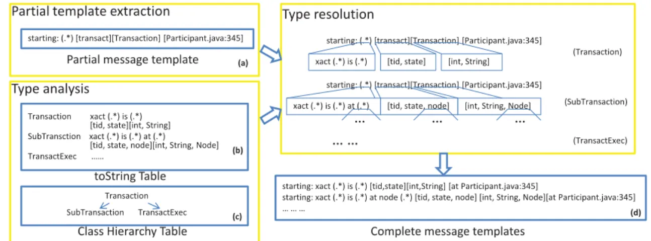
starting: (.*) [transact][Transaction] [Participant.java:345]
Partial message template toString() definitions
starting: xact (.*) is (.*) [tid,state][int,String] [at Participant.java:345] starting: xact (.*) is (.*) at node (.*) [tid, state, node] [int, String, Node] [at Participant.java:345]
Complete message templates AST
Source Code Type hierarchy info
Reverse Index Console Logs
Parsing results
Static source code analysis Runtime log parsing
Figure 3:Using source code information to parse console logs.
underlying structure of the log message. Third, due to class inheritance, the actualtoString() method used in a particular call might be defined in a subclass rather than the base class of the logger object.
Our parsing approach. All three reasons are addressed by our log parsing method that consists of two steps: a static source code analysis step and the runtime log pars-ing step, as Figure 3 illustrates. In particular, we do not claim to handle every situation correctly (despite exten-sive support for language idioms), but we do show that some of the important features used in our results cannot be extracted using existing log parsing techniques.
The static source code analysis step takes program source (and possibly the names of the logger class) as input. In this step, we first generate the source code’s abstract syntax tree (AST) [1], a popular data structure for traversing and analyzing source code. We use the AST implementations built into the open-source Eclipse IDE [25]. We use the AST to identify all method calls on objects of the classes (or their subclasses), recording the filename and line number of the call. Each call gives us only a partial message template, since the template may involve interpolation of objects of nonprimitive types, as in line 1 of the source code excerpt in Figure 1. We then enumerate alltoString() calls in all classes, and look at the string formatting statements in those calls to de-duce the types of variables in message templates, sub-stituting this type information back into the partial tem-plates. We do this recursively until all templates inter-polate only primitive types; if notoString() method can be found for a particular variable anywhere along its inheritance path, we assume that that variable can take on any string value and we do no further semantic interpreta-tion. A single pass can accomplish all of these operations over the AST. The output of the process is the complete message templates, with a data structure containing each message’s template (regular expression), position in the source code, and the names and data types of all variables appearing in the message. We describe the details of the template extraction approach in Appendix A.
To parse the logs, we first compile all message tem-plates into an Apache Lucene [11] reverse index [20], which allows us to quickly associate any log message with the corresponding template. Following established
heuristics in log analysis [17, 30], we construct an index query from each log message by removing all numbers and special symbols. From the list of relevance-ranked candidate results returned by the reverse-index search, we pick the highest-ranked result that allows a regular ex-pression match to succeed against the log message. We note that once the reverse index is constructed (it usu-ally fits in memory), the parsing step is embarrassingly parallel; we implement it as a Hadoop map-reduce job by replicating the index to every worker node and par-titioning the log among the workers, achieving near lin-ear speedup. The map stage performs the reverse-index search; the reduce stage processing depends on the fea-tures to be constructed, and Section 4 shows 2 examples. To summarize, unlike existing log-parsing methods, the fine granularity of structure revealed by our method enables analyses that are traditionally possible only with structured logs. Section 7 discusses the many intrinsic subtleties in source code analysis and log parsing.
4
Feature Creation
This section describes our technique for constructing fea-tures from parsed logs. We focus on two feafea-tures, the state ratio vector and the message count vector, based on state variables and identifiers (see Section 2.1), re-spectively. The state ratio vector is able to capture the aggregated behavior of the system over a time window. The message count vector helps detect problems related to individual operations. Both features describe message groups constructed to have strong correlations among their members. The features faithfully capture these cor-relations, which are often good indicators of runtime problems. Although these features are from the same log, and similar in structure, they are constructed inde-pendently, and have different semantics.
4.1 State variables and state ratio vectors
State variables can appear in a large portion of log mes-sages. In fact, 32% of the log messages from Hadoop and
28%of messages from Darkstar contain state variables. In many systems, during normal execution the relative frequency of each value of a state variable in a time win-dow usually stays the same. For example, in Darkstar, the ratio betweenABORTINGandCOMMITTINGis very stable during normal execution, but changes significantly when
a problem occurs. Notice that the actual number does not matter (as it depends on workload), but the ratio among different values matters.
We construct state ratio vectorsyto encode this corre-lation: Each state ratio vector represents a group of state variables in a time window, while each dimension of the vector corresponds to a distinct state variable value , and the value of the dimension is how many times this state value appears in the time window.
In creating features based on state variables we used an automatic procedure that combined two desiderata: 1) message variables should be frequently reported, but 2) they should range across a small constant number of dis-tinct values that do not depend on the number of mes-sages. Specifically in our experiments, we chose state variables that were reported at least0.2N times, withN the number of messages, and had a number of distinct values not increasing withNfor large values ofN (e.g., more than a few thousand). Our results were not sensitive to the choice of 0.2.
The time window size is also automatically deter-mined. Currently we choose a size that allows the vari-able to appear at least10Dtimes in 80% of all the time windows, whereDis the number of distinct values. This choice of time window allows the variable to appear enough times in each window to make the count sta-tistically significant [4] while keeping the time window small enough to capture transient problems. We tried with other parameters than 10 and 80% and we did not see a significant change in detection results.
We stack alln-dimensionaly’s frommtime windows to construct them×nstate ratio matrixYs.
4.2 Identifiers and message count vectors
Identifiers are also prevalent in logs. For example, almost 50% of messages in HDFS logs contain identifiers. We observe that all log messages reporting the same identi-fier convey a single piece of information about the iden-tifier. For instance, in HDFS, there are multiple log mes-sages about a block when the block is allocated, written, replicated, or deleted. By grouping these messages, we get the message count vector, which is similar to an exe-cution path [8] (from custom instrumentation).
To form the message count vector, we first automati-cally discover identifiers, then group together messages with the same identifier values, and create a vector per group. Each vector dimension corresponds to a different message type, and the value of the dimension tells how many messages of that type appear in the message group. The structure of this feature is analogous to the bag of words model in information retrieval [6]. In our ap-plication, the “document” is the message group. The di-mensions of the vector consist of the union of all useful message types across all groups (analogous to all possi-ble “terms”), and the value of a dimension is the number
Algorithm 1 Message count vector construction
1. Find all message variables reported in the log with the following properties:
a. Reported many times; b. Has many distinct values;
c. Appears in multiple message types. 2. Group messages by values of the variables
chosen above.
3. For each message group, create a message count vectory= [y1, y2, . . . , yn], whereyiis the number of appearances of messages of typei(i= 1. . . n) in the message group.
of appearances of the corresponding message types in a group (corresponding to “term frequency”).
Algorithm 1 summarizes our three-step process for feature construction. We now try to provide intuition be-hind the design choices in this algorithm.
In the first step of the algorithm, we automatically choose identifiers (we do not want to require operators to specify a search key). The intuition is that if a vari-able meets the three criteria in step 1 of Algorithm 1, it is likely to identify object such as transactions. The fre-quency/distinct value pattern of identifiers is very differ-ent from other variables, so it is easy to discover iddiffer-enti- identi-fiers2. We have very few false selections in all data sets, and the small number of false choices is easy to eliminate by a manual examination.
In the second step, the message group essentially de-scribes an execution path, with two major differences. First, not every processing step is necessarily represented in the console logs. Since the logging points are hand chosen by developers, it is reasonable to assume that logged steps should be important for diagnosis. Second, correct ordering of messages is not guaranteed across multiple nodes, due to unsynchronized clocks across many computers. This ordering might be a problem for diagnosing synchronization-related problems, but it is still useful in identifying many kinds of anomalies.
In the third step, we use the bag of words model [6] to represent the message group because: 1) it does not require ordering among terms (message types), and 2) documents with unusual terms are given more weight in document ranking. In our case, the rare log messages are indeed likely to be more important.
We gather all the message count vectors to construct message count matrixYmas anm×nmatrix where each
row is a message count vectory, as described in step 3 of Algorithm 1. Ymhasncolumns, corresponding ton
message types that reported the identifier (analogous to 2Like the state variable case, identifiers are chosen as variables re-ported at least0.2Ntimes, whereNis total number of messages. We also require the variables have at least0.02Ndistinct values, and re-ported in at least 5 distinct messages types.
Feature Rows Columns
Status ratio matrixYs time window state value
Message count matrixYm identifier message type
Table 4:Semantics of rows and columns of features
“terms”).Ymhasmrows, each of which corresponds to
a message group (analogous to “document”).
Although the message count matrix Ym has
com-pletely different semantics from the state ratio matrixYs,
both can be analyzed using matrix-based anomaly detec-tion tools (see Secdetec-tion 5). Table 4 summarizes the se-mantics of the rows and columns of each feature matrix. 4.3 Implementing feature creation algorithms To improve efficiency of our feature generation algo-rithms in map-reduce, we tailored the implementation. The step of discovering state variables and/or identifiers (the first steps in Section 4.1 and 4.2) is a single map-reduce job that calculates the number of distinct values for all variables and determines which variables to in-clude in further feature generation steps. The step of con-structing features from variables is another map-reduce job with log parsing as the map stage and message group-ing as the reduce stage. For the state ratio , we sort messages by time stamp, while for the message count vector, we sort by identifier values. Notice that the map stage (parsing step) only needs to output the required data rather than the entire text message, resulting in huge I/O savings during the data shuffling and sorting before re-duce. Feature creation time is negligible when compared to parsing time.
5
Anomaly Detection
We use anomaly detection methods to find unusual pat-terns in logs. In this way, we can automatically find log segments that are most likely to indicate problems. Given the feature matrices we construct, outlier detec-tion methods can be applied to detect anomalies con-tained in the logs. We have investigated a variety of such methods and have found that Principal Component Anal-ysis (PCA) [5, 16] combined with term-weighting tech-niques from information retrieval [23, 26] yields excel-lent anomaly detection results on both feature matrices, while requiring little parameter tuning.
PCA is a statistical method that captures patterns in high-dimensional data by automatically choosing a set of coordinates—the principal components—that reflect co-variation among the original coordinates. We use PCA to separate out repeating patterns in feature vectors, thereby making abnormal message patterns easier to detect. PCA has runtime linear in the number of feature vectors; there-fore, detection can scale to large logs.
Intuition behind PCA anomaly detection. (The math-challenged may want to skip to the results in Section 6.) By construction, dimensions in our feature vectors are
0 20 40 60 80 100
0 50 100 150
ACTIVE trasactions per sec
CO
MMITTING
tr
a
n
sa
cti
o
n
s
p
A
B
a
y
COMMIT
TING
/sec
ACTIVE per sec
y
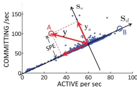
Figure 4: The intuition behind PCA detection with simpli-fied data. We plot only two dimensions from the Darkstar state variable feature. It is easy to see high correlation between these two dimensions. PCA determines the dominant normal pattern, separates it out, and makes it easier to identify anomalies.
Feature data sets n k
Darkstar - message count 18 3
Darkstar - state ratio 6 1
HDFS - message count 28 4
HDFS - state ratio 202 2
Table 5:Low effective dimensionality of feature data.n= Di-mensionality of feature vectory;k= Dimensionality required to capture 95% of variance in the data. In all of our data, we havekn, exhibiting low effective dimensionality.
highly correlated, due to the strong correlation among log messages within a group. We aim to identify abnor-mal vectors that deviate from such correlation patterns. Figure 4 illustrates a simplified example using two di-mensions (number ofACTIVEandCOMMITTINGper sec-ond) from Darkstar state ratio vectors. We see most data points reside close to a straight line (a one-dimensional subspace). In this case, we say the data have low
ef-fective dimensionality. The axisSd captures the strong
correlations between the two dimensions. Intuitively, a data point far from theSd (such as point A) shows un-usual correlation, and thus represents an anomaly. In contrast, point B, although far from most other points, resides close to theSd, and is thus normal. In fact, both
ACTIVEandCOMMITTINGare larger in this case, which simply indicates that the system is busier.
Indeed, we do observe low effective dimensionality in the feature matricesYsandYmin many systems.
Ta-ble 5 showsk, the number of dimensions required to cap-ture 95% of the variance in data3. Intuitively, in the case of the state ratio , when the system is in a stable state, the ratios among different state variable values are roughly constant. For the message count vector, as each dimen-sion corresponds to a certain stage in the program and the stages are determined by the program logic, the mes-sages in a group are correlated. The correlations among messages, determined by the normal program execution, result in highly correlated dimensions for both features.
3This is a common heuristic for determining k in PCA detec-tors [15]; we use this number in all of our experiments.
In summary, PCA captures dominant patterns in data to construct a (low)k-dimensional normal subspaceSd in the original n-dimensional space. The remaining
(n−k)dimensions form the abnormal subspaceSa. By projecting the vectoryonSa(separating out its compo-nent onSd), it is much easier to identify abnormal vec-tors. This forms the basis for anomaly detection [5, 16]. Detecting anomalies. Intuitively, we use the “distance” from the end point of a vectoryto the normal subspace
Sd to determine whether y is abnormal. This can be
formalized by computing the squared prediction error
SPE≡ ya2(the squared length of vectorya), where ya is the projection ofy onto the abnormal subspace Sa, and can be computed asya = (I−PPT)y, where P= [v1,v2, . . . ,vk], is formed by the firstkprincipal
components chosen by PCA algorithm.
As Figure 4 shows, abnormal vectors are typically far away from the normal subspaceSd. Thus, the “detection rule” is simple: we markyis abnormal if
SPE=ya2> Qα, (1)
whereQα denotes the threshold statistic for the SPE residual function at the(1−α)confidence level. Automatically determine detection threshold. To compute Qα we make use of the Q-statistic, a
well-known test statistic for theSPEresidual function [13]. The computed threshold Qα guarantees that the false alarm probability is no more thanαunder the assump-tion that data matrix Y has a multivariate Gaussian distribution. However, as pointed out by Jensen and Solomon [13], and as verified in our empirical work, the Q-statistic is robust even when the underlying distribu-tion of the data differs substantially from Gaussian.
The choice of the confidence parameterαfor anomaly detection has been studied in previous work [16], and we follow standard recommendations in choosingα =
0.001in our experiments. We found that our detection results are not sensitive to this parameter choice. Improving PCA detection results. Our message count vector is constructed in a way similar to the bag-of-words model, so it is natural to consider term weighting tech-niques from information retrieval. We applied Term Fre-quency / Inverse Document FreFre-quency (TF-IDF), a well-established heuristic in information retrieval [23, 26], to pre-process the data. Instead of applying PCA directly to the feature matrixYmwe replace each entryyi,jinYm with a weighted entrywi,j ≡yi,jlog(n/dfj), wheredfj
is total number of message groups that contain thej-th message type. Intuitively, multiplying the original count with the IDF reduces the weight of common message types that appear in most groups, which are less likely to indicate problems. We found this step to be essential for improving detection accuracy.
System Total Log Failed Failed % HDFS 24,396,061 29,636 0.121% Darkstar 1,640,985 35 0.002% Table 6: Parsing accuracy. Parse fails on a message when we cannot find a message template that matches the message and extract message variables.
0 20 40 60 80 100
0 2 4 6 8 10x 10
6
Messages/min
Number of nodes
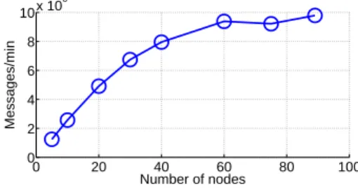
Figure 5: Scalability of log parsing with number of nodes used. The x-axis is the number of nodes used, while the y-axis is the number of messages processed per minute. All nodes are Amazon EC2 high-CPU medium instances. We used the HDFS data set (described in (Table 3) with over 24 million lines. We parsed raw textual logs and generated the message count vec-tor feature (see Section 4.2). Each experiment was repeated 4 times and the reported data point is the mean.
TF-IDF does not apply to the state ratio feature. This is because the state ratio matrix is a dense matrix that is not amenable to an interpretation as a bag-of-words model. However, applying the PCA method directly toYsgives
good results on the state ratio feature.
6
Evaluation and Visualization
We first show the accuracy and scalability achieved by our log parsing method (Section 6.1) and then discuss our experiences with the two real-world systems.
We began our experiments of problem detection with Darkstar, in which both features give simple yet insight-ful results (Section 6.2). Satisfied with these results, we applied our techniques to the much more complex HDFS logs. We also achieve high detection accuracy (Section 6.3). However, the results are less intuitive to system operators and developers, so we developed a de-cision tree visualization method, which summarizes the PCA detection results in a single, intuitive picture (Sec-tion 6.4) that is more operator friendly because the tree resembles the rule-based event processing systems oper-ators use [10].
6.1 Log parsing accuracy and scalability
Accuracy. Table 6 shows that our log parsing method achieves over 99.8% accuracy on both systems. Specif-ically, our technique successfully handled rare messages types, even those that appeared only twice in over 24 mil-lion messages in HDFS. On the contrary, word-frequency based console log analysis tools, such as SLCT [32], do
not recover either of the features we use in this paper. State variables are too common to be separated from con-stant strings by word frequency only. In addition, these tools ignore all rare messages, which are required to con-struct message count vectors.
There are only a few message types that our parser fails to handle. Almost all of these messages contain long string variables. These long strings may overwhelm the constant strings we are searching for, preventing reverse index search from finding the correct message template. However, these messages typically appear at the initial-ization or termination phase of a system (or a subsystem), when the state of the system is dumped to the console. Thus, we did not see any impact of missing these mes-sages on our detection results.
We believe the accuracy of our approach to parsing is essential; only with an accurate parsing system can we extract state variables and identifiers—the basis for our feature construction—from textual logs. Thus, we con-sider the requirement of access to source code to be a small price to pay (especially given that many modules are open-source), given the high quality parsing results that our technique produces.
Scalability. We evaluated the scalability of our log pars-ing approach with a varypars-ing number of EC2 nodes. Fig-ure 5 shows the result: Our log parsing and featFig-ure ex-traction algorithms scale almost linearly with up to about 50 nodes. Even though we parsed all messages gener-ated by 200 HDFS nodes (with aggressive logging) over 48 hours, log parsing only takes less than 3 minutes with 50 nodes, or less than 10 minutes with 10 nodes. When we use more than 60 nodes, the overhead of index dis-semination and job scheduling dominate running time. 6.2 Darkstar experiment results
As mentioned in Section 2.3, we observed high perfor-mance (i.e., client side response time) variability when deploying the Darkstar server on a cloud-computing en-vironment such as EC2 during performance disturbances, especially for CPU contention. We wanted to see if we could understand the reason for this high performance variability solely from console logs. Indeed, we were unfamiliar with Darkstar, so our setting was realistic as the operator often knows little about system internals.
In the experiment, we deployed an unmodified Dark-star0.95distribution on a single node (because the Dark-star version we use supports only one node). DarkDark-star does not log much by default, so we turned on the debug-level logging. We deployed a simple game, DarkMud, provided by the Darkstar team, and created a workload generator that emulated 60 user clients in the DarkMud virtual world performing random operations such as flip-ping switches, picking up and dropflip-ping items. The client emulator recorded the latency of each operation. We ran the experiment for 4800 seconds and injected a
per-formance disturbance by capping the CPU available to Darkstar to 50% of the normal level during time 1400 to 1800.
Detection by state ratio vectors. The only state variable chosen by our feature generation algorithm is state, which is reported in456,996messages (about 28% of all log messages in our data set). It has 8 distinct val-ues, including PREPARING, ACTIVE, COMMITTING,
ABORTINGand so on, so our state ratio matrixYs has
8 columns (dimensions). The time window (automati-cally determined according to Section 4.1) is 3 seconds; we restricted the choice to whole seconds.
Figures 6 (a) and (b) show the results between time 1000 and 2500, where plot (a) displays the average la-tency reported by the client emulator, which acts as a ground truth for evaluating our method, and plot (b) dis-plays the PCA anomaly detection results on the state ra-tio matrixYs. We see that anomalies detected by our
method during the time interval (1400, 1800) match the high client-side latency very well; i.e., the anomalies de-tected in the state ratio matrix correlate very well with the increases in client latency. Comparing the abnormal vectors to the normal vectors, we see that the ratio be-tween number ofABORTINGtoCOMMITTINGincreases from about 1:2000 to about 1:2, indicating that a dispro-portionate number ofABORTINGtransactions are related to the poor client latency.
Generally, the abnormal state ratio may be the cause, symptom, or consequence of the performance degrada-tion. In the Darkstar case, the ratio reflects the cause of the problem: when the system performance gets worse, Darkstar does not adjust transaction timeout accordingly, causing many normal transactions to be aborted and restarted, resulting in further load increase to the system. Notice that a traditional grep-based method does not help in this case for two reasons: 1) As a normal user of Darkstar—without having knowledge about its internals—the transaction states are obscure implemen-tation details. Thus, it is difficult for a user to choose the correct ones from many variables to search for. In contrast, we systematically discover and analyze all state variables. 2)ABORTINGhappens even during normal op-eration times, due to the optimistic concurrency model used in Darkstar, where aborting is used to handle access conflicts. It is not a singleABORTINGmessage, but the ratio ofABORTINGto other values of thestatevariable that captures the problem.
Detection by message count vectors. From Darkstar logs, Algorithm 1 automatically chooses two identifier variables, the transaction id and the asynchronous chan-nel id. Figure 6(c) shows detection results on the mes-sage count vector constructed from the transaction id variable. There are 68,029 transaction ids reported in 18 different message types. Thus, the dimension of matrix
10000 1500 2000 2500 2
4
Latency (sec)
(a) Client latency
← Disturbance starts
← Disturbance ends
Latency
10000 1500 2000 2500
500
Residual
(b) Status ratio vector detection Residual Threshold Alarms
10000 1500 2000 2500
10 20
Time since start (sec)
Residual
(c) Message count vector detection Residual Threshold Alarms
Figure 6: Darkstar detection results. (a) shows that the disturbance injection caused a huge increase in client response time. (b)
shows PCA anomaly detection results on the state ratio vector created from message variablestate. The dashed line shows the
thresholdQα. The solid line with spikes is the SPE calculated according to Eq. (1). The circles denote the anomalous vectors
detected by our method, whose SPE values exceed thresholdQα. (c) shows detection results with the message count vector. The
SPE value of each vector (the solid line) is plotted at the time when the last message of the group occurs.
Ymis68,029×18. By construction, each message count
vector represents a set of operations (message types) oc-curring when executing a transaction. PCA identifies the normal vectors corresponding to a common set of opera-tions (simplified for presentation):{create,join txn,
commit,prepareAndCommit}. Abnormal transactions can deviate from this set by missing a few message types, or having rare message types such as abort txn in-stead of commitandjoin txn. We detected 504 of these as abnormal. To validate our result, we augmented each feature vector using the timestamp of the last mes-sage in that group, and we found that almost all abnormal transactions occur when the disturbance is injected. We see that the anomalies continue to appear (with a smaller frequency) for a short time period after the disturbance stopped due to the queueing effect as the system recov-ered from the disturbance. Notice that the state ratio vec-tor method did not mark the recovery period as abnormal, demonstrating that the message count vector method was more sensitive because it modeled individual operations while state ratio vector method captured only aggregate behavior.
There were no anomalies on the channel id variable during the entire experiment, suggesting that the channel id variable is not related to this performance anomaly.
This result is consistent with the state ratio vector de-tection result. In console logs, it is common that there are several different pieces of information that describe the same system behavior. This commonality suggests an important direction for future research: to exploit multi-source learning algorithms, which combine multiple de-tection results to further improve accuracy.
6.3 Hadoop experiment results
Compared to Darkstar, HDFS is larger scale and the logic is much more complex. In this experiment, we show that we can automatically discover many abnormal behaviors
in HDFS. We generated the HDFS logs by setting up a Hadoop cluster on 203 EC2 nodes and running sample Hadoop map-reduce jobs for 48 hours, generating and processing over 200 TB of random data. We collected over 24 million lines of logs from HDFS.
Detection on message count vector. From HDFS logs, Algorithm 1 automatically chooses one identifier vari-able, the blockid, which is reported in 11,197,954 messages (about 50% of all messages) in 29 message types. Also, there are 575,139distinct blockids re-ported in the log, so the message count matrixYmhas a dimension of575,139×29. The PCA detector gives very good separation between normal and abnormal row vectors in the matrix: Using an automatically determined threshold (Qα in Eq. (1) in Section 5), it can success-fully detect abnormal vectors corresponding to blocks that went through abnormal execution paths.
To further validate our results, we manually labeled each distinct message vector, not only marking them as normal or abnormal, but also determining the type of problems for each vector. The labeling was done by care-fully studying HDFS code and by consulting with local Hadoop experts. We show in the next section that the de-cision tree visualization helps both ourselves and Hadoop developers to understand our results. We emphasize that this labeling step is done only to validate our method—it is not a required step when using our technique. Label-ing half a million vectors is possible because many of the vectors are exactly the same. In fact, there are only 680 distinct vectors, confirming our intuition that most blocks go through a common execution path.
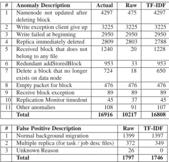
Table 7 shows the manual labels and detection results. We see that the PCA detector can detect a large fraction of anomalies in the data, and significant improvement can be achieved when we preprocess data with TF-IDF , con-firming our expectations from Section 5.
catas-trophic failures; thus, most problems listed in Table 7 only affect performance.
The first anomaly in Table 7 uncovered a bug that has been hidden in HDFS for a long time. In a certain (rel-atively rare) code path, when a block is deleted (due to temporary over-replication), the record on the namenode is not updated until the next write to the block, caus-ing the file system to believe in a replica that no longer exists, which causes subsequent block deletion to fail. Hadoop developers have recently confirmed this bug. This anomaly is hard to find because there is no single error message indicating the problem. However, we dis-cover it because we analyze abnormal execution paths.
We also notice that we do not have the problem that causes confusion in traditional grep based log analysis. In HDFS datanode logs, we see many messages like
#:Got Exception while serving # to #:#. Ac-cording to Apache issue tracking (jira) HADOOP-3678, this is a normal behavior of HDFS: the HDFS data node generates the exception when a HDFS client does not fin-ish reading an entire block before it stops. These excep-tion messages have confused many users, as indicated by multiple discussion threads on the Hadoop user mailing list. While traditional keyword matching (e.g., searching for words like Exception or Error) would have flagged these as errors, our message count method successfully avoids this false positive because this happens too many times to be abnormal.
Our algorithm does report some false positives, which are inevitable in any unsupervised learning algorithm. For example, the second false positive in Table 7 occurs because a few blocks are replicated 10 times instead of 3 times for the majority of blocks. These message groups look suspicious, but Hadoop experts told us that these are normal situations when the map-reduce system is dis-tributing job configuration files to all the nodes. It is in-deed a rare situation compared to the data accesses, but is normal by the system design. Eliminating this type of “rare but normal” false positive requires domain expert knowledge. As a future direction, we are investigating semi-supervised learning techniques that can take opera-tor feedback and further improve our results.
Detection on state ratio vectors. The only state variable chosen in HDFS logs by our feature generation algorithm is the node name. Node name might not sound like a state variable, but as the set of nodes (203 total) are rela-tively fixed in HDFS, and their names meet the criterion of state variable described in Section 4.1. Thus, the state ratio vector feature reduces to per node activity count, a feature well-studied in existing work [12, 17]. As in this previous work, we are able to detect transient workload imbalance, as well as node reboot events. However, our approach is less ad-hoc because the state ratio feature is chosen automatically based on information in the console
# Anomaly Description Actual Raw TF-IDF
1 Namenode not updated after deleting block
4297 475 4297
2 Write exception client give up 3225 3225 3225 3 Write failed at beginning 2950 2950 2950 4 Replica immediately deleted 2809 2803 2788 5 Received block that does not
belong to any file
1240 20 1228
6 Redundant addStoredBlock 953 33 953 7 Delete a block that no longer
exists on data node
724 18 650
8 Empty packet for block 476 476 476
9 Receive block exception 89 89 89
10 Replication Monitor timedout 45 37 45
11 Other anomalies 108 91 107
Total 16916 10217 16808
# False Positive Description Raw TF-IDF
1 Normal background migration 1399 1397 2 Multiple replica (for task / job desc files) 372 349
3 Unknown Reason 26 0
Total 1797 1746
Table 7:Detected anomalies and false positives using PCA on Hadoop message count vector feature. Actual is the number of anomalies labeled manually. Raw is PCA detection result on raw data, TF-IDF is detection result on data preprocessed with TF-IDF and normalized by vector length (Section 5).
log, instead of manually specified.
6.4 Visualizing detection results with decision trees From the point of view of an operator, the transforma-tion underlying PCA is a black box algorithm: it pro-vides no intuitive explanation of the detection results and cannot be interrogated. Human operators need to man-ually examine anomalies to understand the root cause, and PCA itself provides little help in this regard. In this section, we show how to augment PCA-based detection with decision trees to make the results more easily un-derstandable and actionable by operators. The decision tree result resembles the (manually written) rules used in many system-event-processing programs [10], so it is easier for non-machine learning experts. This technique is especially useful for features with many dimensions, such as the message count vector feature in HDFS.
Decision trees have been widely used for classifi-cation. Because decision tree construction works in the original coordinates of the input data, its classifica-tion decisions tend to be easy to visualize and under-stand [34]. Constructing a decision tree requires a train-ing set with class labels. We use the automatically gen-erated PCA detection results (normal vs. abnormal) as class labels, in contrast to the normal use of decision trees. Our decision tree is constructed to explain the un-derlying logic of the detection algorithm, rather than the nature of the dataset.
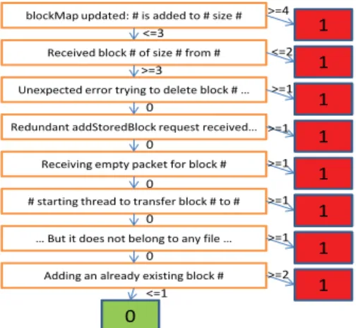
Figure 7 is the decision tree generated using Rapid-Miner [21] from the anomaly detection results of the HDFS log. It clearly shows the most important
mes-0 1
1 1
1 0 0
0
blockMap updated: # is added to # size # Received block # of size # from # Unexpected error trying to delete block # … Redundant addStoredBlock request received…
Receiving empty packet for block # # starting thread to transfer block # to #
… But it does not belong to any file … Adding an already existing block #
1
<=3 >=3
0 0 0
0 0 <=1
>=4 <=2 >=1 >=1 >=1 >=1 >=1 >=2
1
1 1
Figure 7: The decision tree visualization. Each node is the message type string (# is the place holder for variables). The number on the edge is the threshold of message count, gener-ated by the decision tree algorithm. Small boxes contain the labels from PCA, with a red 1 for abnormal and a green 0 for normal.
sage types. For example, the first level shows that if
blockMap(the data structure that keeps block locations) is updated more than 3 times, it is abnormal. This indi-cates the over-replication problem (Anomaly 4 or False Positive 1 in Table 7). The second level shows that if a block is received 2 times or less, it is abnormal; this indi-cates under-replication or block-write failure (Anomaly 2 and 3 in Table 7). Level 3 of the decision tree is related to the bug we discussed in Section 6.3.
In summary, the visualization of results with decision trees helps operators and developers notice types of ab-normal behaviors instead of individual abab-normal events, which can greatly improve the efficiency of finding root causes and preventing future alarms.
7
Discussion
Should we completely replace console logs with struc-tured tracing? There are various such efforts [8, 29]. Progress has been slow, however, mainly because there is no standard for structured tracing embraced by all open source developers. It is also technically difficult to design a global “schema” to accommodate all informa-tion contained in console logs in a structured format4. Even if such a standard existed, manually porting all legacy codes to the schema would be expensive. Auto-matic porting of legacy logging code to structured log-ging would be no simpler than our log parsing. Our feature creation and anomaly detection algorithm can be used withoutlog parsing in systems with structured traces only, and we described a successful example in Sec-tion 2.2
Improving console logs. We have discovered some bad 4syslog is not structured because it uses the free text field heavily.
logging practices that significantly reduced the useful-ness of the console log. Some of them are easy to fix. For example, Facebook’s Cassandra storage system traces all operations of nodes sending messages to each other, but it does not write the sequence number or ID of messages logged. This renders the log almost useless if multiple threads on a single machine are sending messages con-currently. However, just by adding the message ID, our message count method readily applies and would help detect node communication problems.
Another bad logging practice, which has been discov-ered in prior work, is the poor estimate of event severity. Many “FATAL” or “ERROR” events are not as bad as the developer thinks [14, 22]. This mistake is because each developer judges the severity only in the context of his own module instead of in the context of the entire system. As we show in the Hadoop read exception example, our tool, based on the frequency of the events, can provide developers with insight into the real severity of individ-ual events and thus improve qindivid-uality of future logging. Challenges in log parsing. Since we rely on static source code analysis to extract structure from the logs, our method may fail in some cases and fall back on iden-tifying a large chunk of a log message as an unparsed string. For example, if programmers use very general types such asObjectin Java (very rare in practice), our type resolution step fails because there are too many pos-sibilities. We guard against this by limiting the number of descendants of a class to 100, which is large enough to accommodate all logs we studied but small enough to fil-ter out genuine JDK, AWT and Swing classes with many subclasses (such asObject). Features such as generics and mix-ins in modern OO languages provide the mecha-nisms usually needed to avoid having to declare an object in a very general class. In addition, some log messages are undecorated, emitting only a variable of some prim-itive type without any constant label. These messages are usually leftovers from the debugging phase, and we simply ignore these messages.
8
Related Work
Most existing work treats the entire log as a single se-quence of repeating message types and mines it with time series analysis methods. Hellerstein et al. developed a novel method to mine important patterns such as message burst, periodicity and dependencies from SNMP data in an enterprise network [12, 18]. Yamanishi et al. mod-eled syslog sequences as a mixture of Hidden Markov Models (HMM), in order to find messages that are likely to be related to critical failures [35]. Lim et al. analyzed a large-scale enterprise telephony system log with mul-tiple heuristic filters to find messages related to actual failures [17]. Treating a log as a single time series, how-ever, does not perform well in large-scale clusters with