An Elementary Introduction
to Modern Convex Geometry
KEITH BALL
Contents
Preface 1
Lecture 1. Basic Notions 2
Lecture 2. Spherical Sections of the Cube 8
Lecture 3. Fritz John’s Theorem 13
Lecture 4. Volume Ratios and Spherical Sections of the Octahedron 19 Lecture 5. The Brunn–Minkowski Inequality and Its Extensions 25 Lecture 6. Convolutions and Volume Ratios: The Reverse Isoperimetric
Problem 32
Lecture 7. The Central Limit Theorem and Large Deviation Inequalities 37
Lecture 8. Concentration of Measure in Geometry 41
Lecture 9. Dvoretzky’s Theorem 47
Acknowledgements 53
References 53
Index 55
Preface
These notes are based, somewhat loosely, on three series of lectures given by myself, J. Lindenstrauss and G. Schechtman, during the Introductory Workshop in Convex Geometry held at the Mathematical Sciences Research Institute in Berkeley, early in 1996. A fourth series was given by B. Bollob´as, on rapid mixing and random volume algorithms; they are found elsewhere in this book.
The material discussed in these notes is not, for the most part, very new, but the presentation has been strongly influenced by recent developments: among other things, it has been possible to simplify many of the arguments in the light of later discoveries. Instead of giving a comprehensive description of the state of the art, I have tried to describe two or three of the more important ideas that have shaped the modern view of convex geometry, and to make them as accessible
as possible to a broad audience. In most places, I have adopted an informal style that I hope retains some of the spontaneity of the original lectures. Needless to say, my fellow lecturers cannot be held responsible for any shortcomings of this presentation.
I should mention that there are large areas of research that fall under the very general name of convex geometry, but that will barely be touched upon in these notes. The most obvious such area is the classical or “Brunn–Minkowski” theory, which is well covered in [Schneider 1993]. Another noticeable omission is the combinatorial theory of polytopes: a standard reference here is [Brøndsted 1983].
Lecture 1. Basic Notions
The topic of these notes is convex geometry. The objects of study are con-vex bodies: compact, concon-vex subsets of Euclidean spaces, that have nonempty interior. Convex sets occur naturally in many areas of mathematics: linear pro-gramming, probability theory, functional analysis, partial differential equations, information theory, and the geometry of numbers, to name a few.
Although convexity is a simple property to formulate, convex bodies possess a surprisingly rich structure. There are several themes running through these notes: perhaps the most obvious one can be summed up in the sentence: “All convex bodies behave a bit like Euclidean balls.” Before we look at some ways in which this is true it is a good idea to point out ways in which it definitely is not. This lecture will be devoted to the introduction of a few basic examples that we need to keep at the backs of our minds, and one or two well known principles.
The only notational conventions that are worth specifying at this point are the following. We will use| · |to denote the standard Euclidean norm onR
n. For
a bodyK, vol(K) will mean the volume measure of the appropriate dimension. The most fundamental principle in convexity is theHahn–Banach separation theorem, which guarantees that each convex body is an intersection of half-spaces, and that at each point of the boundary of a convex body, there is at least one supporting hyperplane. More generally, ifKandLare disjoint, compact, convex subsets ofR
n, then there is a linear functionalφ:
R
n →
Rfor whichφ(x)< φ(y) wheneverx∈K andy∈L.
The simplest example of a convex body inR
n is the cube, [−1,1]n. This does
not look much like the Euclidean ball. The largest ball inside the cube has radius 1, while the smallest ball containing it has radius √n, since the corners of the cube are this far from the origin. So, as the dimension grows, the cube resembles a ball less and less.
The second example to which we shall refer is then-dimensional regular solid simplex: the convex hull ofn+ 1 equally spaced points. For this body, the ratio of the radii of inscribed and circumscribed balls is n: even worse than for the cube. The two-dimensional case is shown in Figure 1. In Lecture 3 we shall see
Figure 1. Inscribed and circumscribed spheres for ann-simplex.
that these ratios are extremal in a certain well-defined sense. Solid simplices are particular examples of cones. By aconeinR
nwe just mean
the convex hull of a single point and some convex body of dimensionn−1 (Figure 2). In R
n, the volume of a cone of heighthover a base of (n−1)-dimensional
volumeB is Bh/n.
The third example, which we shall investigate more closely in Lecture 4, is the n-dimensional “octahedron”, orcross-polytope: the convex hull of the 2npoints (±1,0,0, . . . ,0), (0,±1,0, . . . ,0), . . . , (0,0, . . . ,0,±1). Since this is the unit ball of the`1 norm onR
n, we shall denote itBn
1. The circumscribing sphere of B1n has radius 1, the inscribed sphere has radius 1/√n; so, as for the cube, the ratio is√n: see Figure 3, left.
Bn
1 is made up of 2npieces similar to the piece whose points have nonnegative coordinates, illustrated in Figure 3, right. This piece is a cone of height 1 over a base, which is the analogous piece inR
n−1. By induction, its volume is
1 n ·
1
n−1 · · · · · 1 2 ·1 =
1 n!, and hence the volume ofB1n is 2n/n!.
(1,0, . . . ,0) (n1, . . . ,1n)
(1,0,0)
(0,1,0) (0,0,1)
Figure 3. The cross-polytope (left) and one orthant thereof (right).
The final example is the Euclidean ball itself, Bn2 =
x∈R
n : n
X
1
x2i ≤1
.
We shall need to know the volume of the ball: call itvn. We can calculate the
surface “area” ofBn
2 very easily in terms of vn: the argument goes back to the
ancients. We think of the ball as being built of thin cones of height 1: see Figure 4, left. Since the volume of each of these cones is 1/ntimes its base area, the surface of the ball has areanvn. The sphere of radius 1, which is the surface of
the ball, we shall denoteSn−1.
To calculatevn, we use integration in spherical polar coordinates. To specify
a pointxwe use two coordinates: r, its distance from 0, andθ, a point on the sphere, which specifies the direction ofx. The pointθplays the role ofn−1 real coordinates. Clearly, in this representation,x=rθ: see Figure 4, right. We can
x
θ
0
write the integral of a function onR n as Z Rn f = Z ∞ r=0 Z
Sn−1
f(rθ) “dθ”rn−1dr. (1.1) The factorrn−1appears because the sphere of radiusrhas arearn−1times that of Sn−1. The notation “dθ” stands for “area” measure on the sphere: its total
mass is the surface area nvn. The most important feature of this measure is its rotational invariance: if A is a subset of the sphere andU is an orthogonal transformation ofR
n, thenU Ahas the same measure as A. Throughout these
lectures we shall normalise integrals like that in (1.1) by pulling out the factor nvn, and write
Z
Rn
f =nvn
Z ∞
0
Z
Sn−1f(rθ)r
n−1dσ(θ)dr
where σ=σn−1 is the rotation-invariant measure onSn−1 of total mass 1. To findvn, we integrate the function
x7→exp
−1 2 n X 1x2i
both ways. This function is at once invariant under rotations and a product of functions depending upon separate coordinates; this is what makes the method work. The integral is
Z Rn f = Z Rn n Y 1
e−x2i/2dx=
n
Y
1
Z ∞
−∞e
−x2i/2dxi
= √2πn. But this equals
nvn
Z ∞
0
Z
Sn−1
e−r2/2rn−1dσ dr=nvn
Z ∞
0 e
−r2/2rn−1dr=v n2n/2Γ
n
2 + 1
. Hence
vn=
πn/2 Γ n2+ 1.
This is extremely small ifnis large. From Stirling’s formula we know that Γ
n
2 + 1
∼√2π e−n/2
n
2
(n+1)/2
, so thatvn is roughly
r
2πe n
n.
To put it another way, the Euclidean ball ofvolume 1 hasradius about
r
n 2πe, which is pretty big.
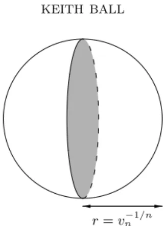
r=v−n1/n
Figure 5. Comparing the volume of a ball with that of its central slice.
This rather surprising property of the ball in high-dimensional spaces is per-haps the first hint that our intuition might lead us astray. The next hint is provided by an answer to the following rather vague question: how is the mass of the ball distributed? To begin with, let’s estimate the (n−1)-dimensional volume of a slice through the centre of the ball of volume 1. The ball has radius
r=vn−1/n
(Figure 5). The slice is an (n−1)-dimensional ball of this radius, so its volume is vn−1rn−1=vn−1
1 vn
(n−1)/n
.
By Stirling’s formula again, we find that the slice has volume about √e when n is large. What are the (n−1)-dimensional volumes of parallel slices? The slice at distancexfrom the centre is an (n−1)-dimensional ball whose radius is √
r2−x2 (whereas the central slice had radiusr), so the volume of the smaller slice is about
√
e
√r2−x2 r
n−1 =√e
1−x 2
r2
(n−1)/2
. Sinceris roughlypn/(2πe), this is about
√
e
1−2πex 2
n
(n−1)/2
≈√eexp(−πex2).
Thus, if we project the mass distribution of the ball of volume 1 onto a single direction, we get a distribution that is approximately Gaussian (normal) with variance 1/(2πe). What is remarkable about this is that the variance does not depend upon n. Despite the fact that the radius of the ball of volume 1 grows like pn/(2πe), almost all of this volume stays within a slab of fixed width: for example, about 96% of the volume lies in the slab
{x∈R
n :−1
2 ≤x1≤12}. See Figure 6.
n= 2
n= 16
n= 120
96%
Figure 6. Balls in various dimensions, and the slab that contains about 96% of each of them.
So the volume of the ball concentrates close to any subspace of dimension n−1. This would seem to suggest that the volume concentrates near the centre of the ball, where the subspaces all meet. But, on the contrary, it is easy to see that, ifnis large, most of the volume of the ball lies near its surface. In objects of high dimension, measure tends to concentrate in places that our low-dimensional intuition considers small. A considerable extension of this curious phenomenon will be exploited in Lectures 8 and 9.
To finish this lecture, let’s write down a formula for the volume of a general body in spherical polar coordinates. LetKbe such a body with 0 in its interior, and for each direction θ ∈ Sn−1 let r(θ) be the radius of K in this direction. Then the volume ofK is
nvn
Z
Sn−1
Z r(θ)
0
sn−1ds dσ=vn
Z
Sn−1
r(θ)ndσ(θ).
This tells us a bit about particular bodies. For example, ifKis the cube [−1,1]n,
whose volume is 2n, the radius satisfies
Z
Sn−1
r(θ)n =2
n
vn ≈
r2n πe
n. So the “average” radius of the cube is about
r
2n πe.
This indicates that the volume of the cube tends to lie in its corners, where the radius is close to √n, not in the middle of its facets, where the radius is close to 1. In Lecture 4 we shall see that the reverse happens forBn
1 and that this has a surprising consequence.
IfK is (centrally) symmetric, that is, if−x∈K wheneverx∈K, thenK is the unit ball of some normk · kK onR
n:
K={x:kxkK ≤1}.
This was already mentioned for the octahedron, which is the unit ball of the`1 norm
kxk=
n
X
1 |xi|. The norm and radius are easily seen to be related by
r(θ) = 1
kθk, forθ∈S
n−1,
sincer(θ) is the largest number r for which rθ ∈K. Thus, for a general sym-metric bodyK with associated normk · k, we have this formula for the volume:
vol(K) =vn
Z
Sn−1
kθk−ndσ(θ).
Lecture 2. Spherical Sections of the Cube
In the first lecture it was explained that the cube is rather unlike a Euclidean ball in R
n: the cube [−1,1]n includes a ball of radius 1 and no more, and is
included in a ball of radius√nand no less. The cube is a bad approximation to the Euclidean ball. In this lecture we shall take this point a bit further. A body like the cube, which is bounded by a finite number of flat facets, is called a polytope. Among symmetric polytopes, the cube has the fewest possible facets, namely 2n. The question we shall address here is this:
If K is a polytope in R
n with m facets, how well can K approximate the
Euclidean ball?
Let’s begin by clarifying the notion of approximation. To simplify matters we shall only consider symmetric bodies. By analogy with the remarks above, we could define the distance between two convex bodiesKandLto be the smallest dfor which there is a scaled copy ofLinsideK and another copy ofL,dtimes as large, containingK. However, for most purposes, it will be more convenient to have an affine-invariant notion of distance: for example we want to regard all parallelograms as the same. Therefore:
Definition. The distance d(K, L) between symmetric convex bodies K and
L is the least positive d for which there is a linear image ˜L of L such that ˜
L⊂K⊂dL˜. (See Figure 7.)
Note that this distance is multiplicative, not additive: in order to get a metric (on the set of linear equivalence classes of symmetric convex bodies) we would need to take logdinstead ofd. In particular, ifK andLare identical thend(K, L) = 1.
˜
L dL˜
K
Figure 7. Defining the distance betweenKandL.
Our observations of the last lecture show that the distance between the cube and the Euclidean ball inR
n isat most √n. It is intuitively clear that it really
is √n, i.e., that we cannot find a linear image of the ball that sandwiches the cube any better than the obvious one. A formal proof will be immediate after the next lecture.
The main result of this lecture will imply that, if a polytope is to have small distance from the Euclidean ball, it must have very many facets: exponentially many in the dimensionn.
Theorem 2.1. LetKbe a(symmetric)polytope inR
n withd(K, Bn
2) =d. Then
K has at leasten/(2d2) facets. On the other hand,for eachn,there is a polytope
with4n facets whose distance from the ball is at most 2.
The arguments in this lecture, including the result just stated, go back to the early days of packing and covering problems. A classical reference for the subject is [Rogers 1964].
Before we embark upon a proof of Theorem 2.1, let’s look at a reformulation that will motivate several more sophisticated results later on. A symmetric convex body in R
n with m pairs of facets can be realised as an n-dimensional
slice (through the centre) of the cube in R
m. This is because such a body is
the intersection of m slabs in R
n, each of the form {x:|hx, vi| ≤1}, for some
nonzero vectorvin R
n. This is shown in Figure 8.
ThusKis the set{x:|hx, vii| ≤1 for 1≤i≤m}, for some sequence (vi)m1 of vectors inR
n. The linear map
T :x7→(hx, v1i, . . . ,hx, vmi)
embeds R
n as a subspace H of
R
m, and the intersection of H with the cube
[−1,1]mis the set of points y in H for which|y
i| ≤1 for each coordinatei. So
this intersection is the image ofK underT. Conversely, anyn-dimensional slice of [−1,1]m is a body with at most m pairs of faces. Thus, the result we are
aiming at can be formulated as follows: The cube inR
m has almost spherical sections whose dimensionnis roughly
Figure 8. Any symmetric polytope is a section of a cube.
In Lecture 9 we shall see that all symmetricm-dimensional convex bodies have almost spherical sections of dimension about logm. As one might expect, this is a great deal more difficult to prove for general bodies than just for the cube.
For the proof of Theorem 2.1, let’s forget the symmetry assumption again and just ask for a polytope
K={x:hx, vii ≤1 for 1≤i≤m}
withmfacets for which
B2n⊂K⊂dB2n.
What do these inclusions say about the vectors (vi)? The first implies that each
vi has length at most 1, since, if not, vi/|vi| would be a vector in B2n but not in K. The second inclusion says that ifx does not belong todB2n thenxdoes not belong toK: that is, if|x|> d, there is an ifor which hx, vii>1. This is
equivalent to the assertion that for every unit vectorθthere is anifor which hθ, vii ≥
1 d.
Thus our problem is to look for as few vectors as possible, v1, v2, . . . , vm, of length at most 1, with the property that for every unit vectorθthere is somevi
withhθ, vii ≥1/d. It is clear that we cannot do better than to look for vectors
of length exactly 1: that is, that we may assume that all facets of our polytope touch the ball. Henceforth we shall discuss only such vectors.
For a fixed unit vectorv andε∈[0,1), the setC(ε, v) ofθ∈Sn−1for which hθ, vi ≥ε is called aspherical cap(or just a cap); when we want to be precise, we will call it theε-cap aboutv. (Note thatεdoes not refer to the radius!) See Figure 9, left.
We want everyθ∈Sn−1to belong to at least one of the (1/d)-caps determined
by the (vi). So our task is to estimate the number of caps of a given size needed
to cover the entire sphere. The principal tool for doing this will be upper and lower estimates for the area of a spherical cap. As in the last lecture, we shall
0
ε v v
r
Figure 9. Left: ε-capC(ε, v)aboutv. Right: cap of radiusraboutv.
measure this area as a proportion of the sphere: that is, we shall use σn−1 as
our measure. Clearly, if we show that each cap occupies only a small proportion of the sphere, we can conclude that we need plenty of caps to cover the sphere. What is slightly more surprising is that once we have shown that spherical caps are not too small, we will also be able to deduce that we can cover the sphere without using too many.
In order to state the estimates for the areas of caps, it will sometimes be convenient to measure the size of a cap in terms of its radius, instead of using theεmeasure. The cap of radiusraboutv is
θ∈Sn−1:|θ−v| ≤r
as illustrated in Figure 9, right. (In defining the radius of a cap in this way we are implicitly adopting a particular metric on the sphere: the metric induced by the usual Euclidean norm onR
n.) The two estimates we shall use are given in
the following lemmas.
Lemma 2.2 (Upper bound for spherical caps). For 0 ≤ ε < 1, the cap
C(ε, u)onSn−1 has measure at moste−nε2/2.
Lemma 2.3 (Lower bound for spherical caps). For 0≤r≤2, a cap of radius ron Sn−1 has measure at least 1
2(r/2)n−1. We can now prove Theorem 2.1.
Proof. Lemma 2.2 implies the first assertion of Theorem 2.1 immediately. If
K is a polytope inR
n withmfacets and ifBn
2 ⊂K⊂dB2n, we can findmcaps
C(1d, vi) coveringSn−1. Each covers at moste−n/(2d 2)
of the sphere, so m≥exp
n
2d2
.
To get the second assertion of Theorem 2.1 from Lemma 2.3 we need a little more argument. It suffices to find m= 4n pointsv1, v2, . . . , vmon the sphere so
that the caps of radius 1 centred at these points cover the sphere: see Figure 10. Such a set of points is called a 1-netfor the sphere: every point of the sphere is
1
1 2 0
Figure 10. The 12-cap has radius 1.
within distance 1 of somevi. Now, if we choose a set of points on the sphere any
two of which are atleastdistance 1 apart, this set cannot have too many points. (Such a set is called 1-separated.) The reason is that the caps of radius 12 about these points will be disjoint, so the sum of their areas will be at most 1. A cap of radius 12 has area at least 14n, so the numbermof these caps satisfiesm≤4n. This does the job, because a maximal 1-separated set is automatically a 1-net: if we can’t add any further points that are at least distance 1 from all the points we have got, it can only be because every point of the sphere iswithindistance 1 of at least one of our chosen points. So the sphere has a 1-net consisting of only 4n points, which is what we wanted to show.
Lemmas 2.2 and 2.3 are routine calculations that can be done in many ways. We leave Lemma 2.3 to the dedicated reader. Lemma 2.2, which will be quoted throughout Lectures 8 and 9, is closely related to the Gaussian decay of the volume of the ball described in the last lecture. At least for smallishε(which is the interesting range) it can be proved as follows.
Proof. The proportion of Sn−1 belonging to the cap C(ε, u) equals the
pro-portion of the solid ball that lies in the “spherical cone” illustrated in Figure 11.
0
ε
√ 1−ε2
As is also illustrated, this spherical cone is contained in a ball of radius√1−ε2 (if ε≤1/√2), so the ratio of its volume to that of the ball is at most
1−ε2n/2≤e−nε2/2.
In Lecture 8 we shall quote the upper estimate for areas of caps repeatedly. We shall in fact be using yet a third way to measure caps that differs very slightly from the C(ε, u) description. The reader can easily check that the preceding argument yields the same estimatee−nε2/2 for this other description.
Lecture 3. Fritz John’s Theorem
In the first lecture we saw that the cube and the cross-polytope lie at distance at most√nfrom the Euclidean ball inR
n, and that for the simplex, the distance
is at mostn. It is intuitively clear that these estimates cannot be improved. In this lecture we shall describe a strong sense in which this is as bad as things get. The theorem we shall describe was proved by Fritz John [1948].
John considered ellipsoids inside convex bodies. If (ej)n1 is an orthonormal basis ofR
n and (α
j) are positive numbers, the ellipsoid
(
x:
n
X
1
hx, eji2
α2j ≤1
)
has volume vn
Q
αj. John showed that each convex body contains a unique
ellipsoid of largest volume and, more importantly, hecharacterised it. He showed that ifK is a symmetric convex body inR
n andE is its maximal ellipsoid then
K⊂√nE.
Hence, after an affine transformation (one takingE toB2n) we can arrange that Bn2 ⊂K⊂√nB2n.
A nonsymmetricK may requirenB2n, like the simplex, rather than√nB2n. John’s characterisation of the maximal ellipsoid is best expressed after an affine transformation that takes the maximal ellipsoid toBn
2. The theorem states thatB2nis the maximal ellipsoid inKif a certain condition holds—roughly, that there be plenty of points of contact between the boundary ofK and that of the ball. See Figure 12.
Theorem 3.1 (John’s Theorem). Each convex body K contains an unique ellipsoid of maximal volume. This ellipsoid is Bn
2 if and only if the following conditions are satisfied: Bn
2 ⊂ K and (for some m) there are Euclidean unit vectors(ui)m1 on the boundary ofK and positive numbers (ci)m1 satisfying
X
ciui= 0 (3.1)
and X
cihx, uii2=|x|2 for each x∈R
Figure 12. The maximal ellipsoid touches the boundary at many points.
According to the theorem the points at which the sphere touches∂Kcan be given a mass distribution whose centre of mass is the origin and whose inertia tensor is the identity matrix. Let’s see where these conditions come from. The first condition, (3.1), guarantees that the (ui) do not all lie “on one side of the sphere”. If they did, we could move the ball away from these contact points and blow it up a bit to obtain a larger ball inK. See Figure 13.
The second condition, (3.2), shows that the (ui) behave rather like an
or-thonormal basis in that we can resolve the Euclidean norm as a (weighted) sum of squares of inner products. Condition (3.2) is equivalent to the statement that
x=Xcihx, uiiui for allx.
This guarantees that the (ui) do not all lie close to a proper subspace ofR
n. If
they did, we could shrink the ball a little in this subspace and expand it in an orthogonal direction, to obtain a larger ellipsoid insideK. See Figure 14.
Condition (3.2) is often written in matrix (or operator) notation as
X
ciui⊗ui=In (3.3)
where In is the identity map on R
n and, for any unit vector u, u⊗u is the
rank-one orthogonal projection onto the span ofu, that is, the mapx7→ hx, uiu. The trace of such an orthogonal projection is 1. By equating the traces of the
Figure 14. An ellipsoid (solid circle) whose contact points are all near one plane can grow.
matrices in the preceding equation, we obtain
X
ci=n.
In the case of asymmetric convex body, condition (3.1) is redundant, since we can take any sequence (ui) of contact points satisfying condition (3.2) and
replace eachui by the pair±ui each with half the weight of the original.
Let’s look at a few concrete examples. The simplest is the cube. For this body the maximal ellipsoid isB2n, as one would expect. The contact points are the standard basis vectors (e1, e2, . . . , en) of R
n and their negatives, and they
satisfy
n
X
1
ei⊗ei=In.
That is, one can take all the weightsci equal to 1 in (3.2). See Figure 15.
The simplest nonsymmetric example is the simplex. In general, there is no natural way to place a regular simplex inR
n, so there is no natural description of
the contact points. Usually the best way to talk about ann-dimensional simplex is to realise it in R
n+1: for example as the convex hull of the standard basis
e1
e2
Figure 16. K is contained in the convex body determined by the hyperplanes tangent to the maximal ellipsoid at the contact points.
vectors inR
n+1. We leave it as an exercise for the reader to come up with a nice description of the contact points.
One may get a bit more of a feel for the second condition in John’s Theorem by interpreting it as a rigidity condition. A sequence of unit vectors (ui) satisfying
the condition (for some sequence (ci)) has the property that ifT is a linear map of determinant 1, not all the imagesT uican have Euclidean norm less than 1.
John’s characterisation immediately implies the inclusion mentioned earlier: ifK is symmetric andE is its maximal ellipsoid thenK⊂√nE. To check this we may assumeE =Bn
2. At each contact point ui, the convex bodiesB2n and
K have the same supporting hyperplane. ForB2n, the supporting hyperplane at any pointuis perpendicular tou. Thus if x∈K we havehx, uii ≤1 for eachi,
and we conclude thatK is a subset of the convex body C={x∈R
n :hx, u
ii ≤1 for 1≤i≤m}. (3.4)
An example of this is shown in Figure 16.
In the symmetric case, the same argument shows that for eachx∈Kwe have |hx, uii| ≤1 for eachi. Hence, forx∈K,
|x|2=Xcihx, uii2≤
X
ci=n.
So|x| ≤√n, which is exactly the statementK⊂√n B2n. We leave as a slightly trickier exercise the estimate|x| ≤nin the nonsymmetric case.
Proof of John’s Theorem. The proof is in two parts, the harder of which
is to show that if Bn
2 is an ellipsoid of largest volume, then we can find an appropriate system of weights on the contact points. The easier part is to show that if such a system of weights exists, thenB2nis theuniqueellipsoid of maximal volume. We shall describe the proof only in the symmetric case, since the added complications in the general case add little to the ideas.
We begin with the easier part. Suppose there are unit vectors (ui) in∂Kand
numbers (ci) satisfying X
ciui⊗ui=In.
Let
E=
x:
n
X
1
hx, eji2 α2j ≤1
be an ellipsoid inK, for some orthonormal basis (ej) and positiveαj. We want
to show that
n
Y
1
αj≤1
and that the product is equal to 1 only ifαj = 1 for allj.
SinceE ⊂Kwe have that for eachithe hyperplane{x:hx, uii= 1}does not
cutE. This implies that eachui belongs to thepolar ellipsoid
y:
n
X
1
α2jhy, eji2≤1
.
(The reader unfamiliar with duality is invited to check this.) So, for eachi,
n
X
j=1
α2jhui, eji2≤1.
Hence X
i
ci
X
j
α2jhui, eji2≤
X
ci=n.
But the left side of the equality is just Pjα2j, because, by condition (3.2), we
have X
i
cihui, eji2=|ej|2= 1
for eachj. Finally, the fact that the geometric mean does not exceed the arith-metic mean (the AM/GM inequality) implies that
Yα2j
1/n≤ 1
n
X
α2j ≤1,
and there is equality in the first of these inequalities only if allαjare equal to 1.
We now move to the harder direction. Suppose Bn
2 is an ellipsoid of largest volume inK. We want to show that there is a sequence of contact points (ui)
and positive weights (ci) with 1 nIn =
1 n
X
ciui⊗ui.
We already know that, if this is possible, we must have
Xci
So our aim is to show that the matrixIn/ncan be written as a convex
combina-tion of (a finite number of) matrices of the formu⊗u, where eachuis a contact point. Since the space of matrices is finite-dimensional, the problem is simply to show that In/n belongs to the convex hull of the set of all such rank-one
matrices,
T ={u⊗u:uis a contact point}.
We shall aim to get a contradiction by showing that ifIn/nisnot in T, we can
perturb the unit ball slightly to get a new ellipsoid inK of larger volume than the unit ball.
Suppose thatIn/nis not inT. Apply the separation theorem in the space of
matrices to get a linear functionalφ(on this space) with the property that φ
I nn
< φ(u⊗u) (3.5) for each contact pointu. Observe thatφcan be represented by ann×nmatrix H = (hjk), so that, for any matrixA= (ajk),
φ(A) =X
jk
hjkajk.
Since all the matricesu⊗uandIn/nare symmetric, we may assume the same
for H. Moreover, since these matrices all have the same trace, namely 1, the inequality φ(In/n) < φ(u⊗u) will remain unchanged if we add a constant to
each diagonal entry ofH. So we may assume that the trace ofH is 0: but this says precisely thatφ(In) = 0.
Hence, unless the identity has the representation we want, we have found a symmetric matrixH with zero trace for which
X
jk
hjk(u⊗u)jk>0
for every contact pointu. We shall use thisHto build a bigger ellipsoid insideK. Now, for each vectoru, the expression
X
jk
hjk(u⊗u)jk
is just the numberuTHu. For sufficiently smallδ >0, the set
Eδ =
x∈R
n :xT(I
n+δH)x≤1
is an ellipsoid and asδ tends to 0 these ellipsoids approach Bn
2. If uis one of the original contact points, then
uT(In+δH)u= 1 +δuTHu >1,
soudoes not belong toEδ. Since the boundary ofKis compact (and the function
δis sufficiently small. Thus, for suchδ, the ellipsoidEδ is strictly insideK and
some slightly expanded ellipsoid is insideK.
It remains to check that eachEδ has volume at least that ofB2n. If we denote by (µj) the eigenvalues of the symmetric matrixIn+δH, the volume of Eδ is
vn
Q
µj, so the problem is to show that, for each δ, we have
Q
µj ≤1. What
we know is thatPµj is the trace ofIn+δH, which isn, since the trace ofH is
0. So the AM/GM inequality again gives
Y
µ1j/n≤ 1 n
X
µj≤1,
as required.
There is an analogue of John’s Theorem that characterises the unique ellipsoid of minimal volume containing a given convex body. (The characterisation is almost identical, guaranteeing a resolution of the identity in terms of contact points of the body and the Euclidean sphere.) This minimal volume ellipsoid theorem can be deduced directly from John’s Theorem by duality. It follows that, for example, the ellipsoid of minimal volume containing the cube [−1,1]n
is the obvious one: the ball of radius√n. It has been mentioned several times without proof that the distance of the cube from the Euclidean ball in R
n is
exactly√n.We can now see this easily: the ellipsoid of minimal volume outside the cube has volume √nntimes that of the ellipsoid of maximal volume inside the cube. So we cannot sandwich the cube between homothetic ellipsoids unless the outer one is at least√ntimes the inner one.
We shall be using John’s Theorem several times in the remaining lectures. At this point it is worth mentioning important extensions of the result. We can view John’s Theorem as a description of those linear maps from Euclidean space to a normed space (whose unit ball isK) that have largest determinant, subject to the condition that they have norm at most 1: that is, that they map the Euclidean ball intoK. There are many other norms that can be put on the space of linear maps. John’s Theorem is the starting point for a general theory that builds ellipsoids related to convex bodies by maximising determinants subject to other constraints on linear maps. This theory played a crucial role in the development of convex geometry over the last 15 years. This development is described in detail in [Tomczak-Jaegermann 1988].
Lecture 4. Volume Ratios and Spherical Sections of the
Octahedron
In the second lecture we saw that then-dimensional cube has almost spherical sections of dimension about lognbut not more. In this lecture we will examine the corresponding question for then-dimensional cross-polytope Bn1. In itself, this body is as far from the Euclidean ball as is the cube inR
n: its distance from
almost spherical sections whose dimension is about12n. We shall deduce this from what is perhaps an even more surprising statement concerning intersections of bodies. Recall that B1n contains the Euclidean ball of radius √1
n. If U is an
orthogonal transformation ofR
n thenU Bn
1 also contains this ball and hence so does the intersectionB1n∩U B1n. But, whereasB1n does not lie in any Euclidean ball of radius less than 1, we have the following theorem [Kaˇsin 1977]:
Theorem 4.1. For each n, there is an orthogonal transformationU for which the intersection Bn
1 ∩U B1n is contained in the Euclidean ball of radius 32/√n (and contains the ball of radius1/√n).
(The constant 32 can easily be improved: the important point is that it is inde-pendent of the dimensionn.) The theorem states that the intersection of just two copies of then-dimensional octahedron may be approximately spherical. Notice that if we tried to approximate the Euclidean ball by intersecting rotated copies of the cube, we would need exponentially many in the dimension, because the cube has only 2nfacets and our approximation needs exponentially many facets. In contrast, the octahedron has a much larger number of facets, 2n: but of course
we need to do a lot more than just count facets in order to prove Theorem 4.1. Before going any further we should perhaps remark that the cube has a property that corresponds to Theorem 4.1. IfQis the cube andU is the same orthogonal transformation as in the theorem, the convex hull
conv(Q∪U Q) is at distance at most 32 from the Euclidean ball.
In spirit, the argument we shall use to establish Theorem 4.1 is Kaˇsin’s original one but, following [Szarek 1978], we isolate the main ingredient and we organise the proof along the lines of [Pisier 1989]. Some motivation may be helpful. The ellipsoid of maximal volume inside Bn
1 is the Euclidean ball of radius √1n. (See
Figure 3.) There are 2npoints of contact between this ball and the boundary of
B1n: namely, the points of the form
±1
n,± 1 n, . . . ,±
1 n
, one in the middle of each facet ofBn
1. The vertices, (±1,0,0, . . . ,0), . . . ,(0,0, . . . ,0,±1), are the points ofBn
1 furthest from the origin. We are looking for a rotationU B1n whose facets chop off the spikes ofBn
1 (or vice versa). So we want to know that the points ofB1n at distance about 1/√nfrom the origin are fairly typical, while those at distance 1 are atypical.
For a unit vectorθ∈Sn−1, letr(θ) be the radius ofB1n in the directionθ, r(θ) = 1
kθk1 =
Xn1 |θi|
−1In the first lecture it was explained that the volume ofBn1 can be written vn
Z
Sn−1
r(θ)ndσ and that it is equal to 2n/n!. Hence
Z
Sn−1
r(θ)ndσ= 2
n
n!vn ≤
2 √
n
n
.
Since the average ofr(θ)n is at most 2/√nn, the value ofr(θ) cannot often be much more than 2/√n. This feature ofBn
1 is captured in the following definition of Szarek.
Definition. LetK be a convex body inR
n. Thevolume ratio ofK is
vr(K) =
vol(K) vol(E)
1/n
, whereE is the ellipsoid of maximal volume inK. The preceding discussion shows that vr(Bn
1)≤2 for alln. Contrast this with the cube in R
n, whose volume ratio is about√n/2. The only property of Bn
1 that we shall use to prove Kaˇsin’s Theorem is that its volume ratio is at most 2. For convenience, we scale everything up by a factor of√nand prove the following.
Theorem 4.2. Let K be a symmetric convex body in R
n that contains the
Euclidean unit ballBn
2 and for which
vol(K) vol(Bn
2)
1/n
=R.
Then there is an orthogonal transformation U ofR
n for which
K∩U K⊂8R2B2n.
Proof. It is convenient to work with the norm onR
n whose unit ball isK. Let
k · kdenote this norm and| · | the standard Euclidean norm. Notice that, since Bn
2 ⊂K, we havekxk ≤ |x| for allx∈R
n.
The radius of the body K∩U K in a given direction is the minimum of the radii of K and U K in that direction. So the norm corresponding to the body K∩U K is themaximum of the norms corresponding toK and U K. We need to find an orthogonal transformationU with the property that
max (kU θk,kθk)≥ 1 8R2
for everyθ∈Sn−1. Since the maximum of two numbers is at least their average,
it will suffice to findU with
kU θk+kθk
2 ≥
1
For eachx∈R
n writeN(x) for the average 1
2(kU xk+kxk). One sees imme-diately that N is a norm (that is, it satisfies the triangle inequality) and that N(x)≤ |x|for everyx, sinceU preserves the Euclidean norm. We shall show in a moment that there is aU for which
Z
Sn−1
1
N(θ)2ndσ≤R
2n. (4.1)
This says that N(θ) is large on average: we want to deduce that it is large everywhere.
Letφbe a point of the sphere and writeN(φ) =t, for 0< t≤1. The crucial point will be that, ifθis close toφ, thenN(θ) cannot be much more thant. To be precise, if|θ−φ| ≤tthen
N(θ)≤N(φ) +N(θ−φ)≤t+|θ−φ| ≤2t.
Hence, N(θ) is at most 2t for every θ in a spherical cap of radius t about φ. From Lemma 2.3 we know that this spherical cap has measure at least
1 2
t2
n−1 ≥t2
n.
So 1/N(θ)2n is at least 1/(2t)2n on a set of measure at least (t/2)n. Therefore
Z
Sn−1
1
N(θ)2ndσ≥
1 (2t)2n
t2
n= 1
23ntn.
By (4.1), the integral is at mostR2n, sot≥1/(8R2). Thus our arbitrary point φsatisfies
N(φ)≥ 1 8R2.
It remains to findU satisfying (4.1). Now, for anyθ, we have N(θ)2=
kU θk+kθk 2
2
≥ kU θk kθk, so it will suffice to find aU for which
Z
Sn−1
1
kU θknkθkndσ≤R2
n. (4.2)
The hypothesis on the volume ofK can be written in terms of the norm as
Z
Sn−1
1
kθkndσ=R n.
The group of orthogonal transformations carries an invariant probability mea-sure. This means that we can average a function over the group in a natural way. In particular, iff is a function on the sphere andθ is some point on the
sphere, the average over orthogonalU of the valuef(U θ) is just the average of f on the sphere: averaging overU mimics averaging over the sphere:
aveUf(U θ) =
Z
Sn−1
f(φ)dσ(φ). Hence,
aveU
Z
Sn−1
1
kU θkn.kθkndσ(θ) =
Z
Sn−1
aveU 1 kU θkn
1
kθkndσ(θ)
=
Z
Sn−1
Z
Sn−1
1
kφkndσ(φ)
1
kθkndσ(θ)
=
Z
Sn−1
1
kθkndσ(θ)
2
=R2n.
Since the average over allU of the integral is at mostR2n, there is at least one U for which the integral is at mostR2n. This is exactly inequality (4.2).
The choice of U in the preceding proof is a random one. The proof does not in any way tell us how to find an explicitU for which the integral is small. In the case of a general body K, this is hardly surprising, since we are assuming nothing about how the volume ofK is distributed. But, in view of the earlier remarks about facets ofBn
1 chopping off spikes ofU B1n, it is tempting to think that for the particular bodyBn
1 we might be able to write down an appropriate
U explicitly. In two dimensions the best choice ofU is obvious: we rotate the diamond through 45◦ and after intersection we have a regular octagon as shown in Figure 17.
The most natural way to try to generalise this to higher dimensions is to look for aU such that each vertex ofU B1n is exactly aligned through the centre of a facet ofBn
1: that is, for each standard basis vectorei ofR
n,U e
i is a multiple of
one of the vectors (±n1, . . . ,±1n). (The multiple is√nsinceU ei has length 1.) Thus we are looking for ann×n orthogonal matrixU each of whose entries is
B12 UB12 B12∩UB12
±1/√n. Such matrices, apart from the factor√n, are calledHadamard matrices. In what dimensions do they exist? In dimensions 1 and 2 there are the obvious
(1) and 1
√
2 √12 1
√
2 −√12
!
.
It is not too hard to show that in larger dimensions a Hadamard matrix cannot exist unless the dimension is a multiple of 4. It is an open problem to determine whether they exist in all dimensions that are multiples of 4. They are known to exist, for example, if the dimension is a power of 2: these examples are known as the Walsh matrices.
In spite of this, it seems extremely unlikely that one might prove Kaˇsin’s Theorem using Hadamard matrices. The Walsh matrices certainly do not give anything smaller than n−1/4; pretty miserable compared with n−1/2. There are some good reasons, related to Ramsey theory, for believing that one cannot expect to find genuinely explicit matrices of any kind that would give the right estimates.
Let’s return to the question with which we opened the lecture and see how Theorem 4.1 yields almost spherical sections of octahedra. We shall show that, for each n, the 2n-dimensional octahedron has an n-dimensional slice which is within distance 32 of the (n-dimensional) Euclidean ball. By applying the argument of the theorem toBn
1, we obtain ann×northogonal matrixU such that
kU xk1+kxk1≥
√
n 16|x| for every x ∈ R
n, where k · k1 denotes the `
1 norm. Now consider the map
T :R
n →
R
2n with matrix U I
. For eachx∈R
n, the norm ofT xin`2n
1 is kT xk1=kU xk1+kxk1≥
√
n 16|x|. On the other hand, the Euclidean norm ofT xis
|T x|=p|U x|2+|x|2=√2|x|. So, ifybelongs to the imageTR
n, then, settingy=T x,
kyk1≥
√
n 16|x|=
√
n 16√2|y|=
√ 2n 32 |y|.
By the Cauchy–Schwarz inequality, we havekyk1≤√2n|y|, so the slice ofB2n
1 by the subspaceTR
n has distance at most 32 fromBn
2, as we wished to show. A good deal of work has been done on embedding of other subspaces ofL1 into `1-spaces of low dimension, and more generally subspaces of Lp into low-dimensional `p, for 1 < p < 2. The techniques used come from probability
theory: p-stable random variables, bootstrapping of probabilities and deviation estimates. We shall be looking at applications of the latter in Lectures 8 and 9.
The major references are [Johnson and Schechtman 1982; Bourgain et al. 1989; Talagrand 1990].
Volume ratios have been studied in considerable depth. They have been found to be closely related to the so-called cotype-2 property of normed spaces: this re-lationship is dealt with comprehensively in [Pisier 1989]. In particular, Bourgain and Milman [1987] showed that a bound for the cotype-2 constant of a space implies a bound for the volume ratio of its unit ball. This demonstrated, among other things, that there is a uniform bound for the volume ratios of slices of octahedra of all dimensions. A sharp version of this result was proved in [Ball 1991]: namely, that for eachn,Bn
1 has largest volume ratio among the balls of
n-dimensional subspaces ofL1. The proof uses techniques that will be discussed in Lecture 6.
This is a good point to mention a result of Milman [1985] that looks super-ficially like the results of this lecture but lies a good deal deeper. We remarked that while we can almost get a sphere by intersecting two copies ofBn1, this is very far from possible with two cubes. Conversely, we can get an almost spher-ical convex hull of two cubes but not of two copies of Bn
1. The QS-Theorem (an abbreviation for “quotient of a subspace”) states that if we combine the two operations, intersection and convex hull, we can get a sphere no matter what body we start with.
Theorem 4.3 (QS-Theorem). There is a constant M (independent of ev-erything) such that,for any symmetric convex bodyK of any dimension, there are linear maps Q and S and an ellipsoid E with the following property: if
˜
K= conv(K∪QK),then
E ⊂K˜ ∩SK˜ ⊂ME.
Lecture 5. The Brunn–Minkowski Inequality
and Its Extensions
In this lecture we shall introduce one of the most fundamental principles in convex geometry: the Brunn–Minkowski inequality. In order to motivate it, let’s begin with a simple observation concerning convex sets in the plane. LetK⊂R
2 be such a set and consider its slices by a family of parallel lines, for example those parallel to they-axis. If the linex=rmeetsK, call the length of the slicev(r). The graph ofv is obtained by shakingKdown onto thex-axis like a deck of cards (of different lengths). This is shown in Figure 18. It is easy to see that the functionvis concave on its support. Towards the end of the last century, Brunn investigated what happens if we try something similar in higher dimensions.
Figure 19 shows an example in three dimensions. The central, hexagonal, slice has larger volume than the triangular slices at the ends: each triangular slice can be decomposed into four smaller triangles, while the hexagon is a union of six such triangles. So our first guess might be that the slice area is a concave
v(x)
K
Figure 18. Shaking down a convex body.
function, just as slice length was concave for sets in the plane. That this is not always so can be seen by considering slices of a cone, parallel to its base: see Figure 20.
Since the area of a slice varies as the square of its distance from the cone’s vertex, the area function obtained looks like a piece of the curvey=x2, which is certainly not concave. However, it is reasonable to guess that the cone is an extremal example, since it is “only just” a convex body: its curved surface is “made up of straight lines”. For this body, the square root of the slice function just manages to be concave on its support (since its graph is a line segment). So our second guess might be that for a convex body inR
3, a slice-area function has a square-root that is concave on its support. This was proved by Brunn using an elegant symmetrisation method. His argument works just as well in higher dimensions to give the following result for the (n−1)-dimensional volumes of slices of a body inR
n.
Figure 19. A polyhedron in three dimensions. The faces at the right and left are parallel.
x
Figure 20. The area of a cone’s section increases withx2.
Theorem 5.1 (Brunn). Let K be a convex body in R
n, letu be a unit vector
inR
n, and for eachr letH
r be the hyperplane
{x∈R
n :hx, ui=r}.
Then the function
r7→vol (K∩Hr)1/(n−1)
is concave on its support.
One consequence of this is that if K is centrally symmetric, the largest slice perpendicular to a given direction is the central slice (since an even concave function is largest at 0). This is the situation in Figure 19.
Brunn’s Theorem was turned from an elegant curiosity into a powerful tool by Minkowski. His reformulation works in the following way. Consider three parallel slices of a convex body inR
n at positionsr,sandt, wheres= (1−λ)r+λtfor
someλ∈(0,1). This is shown in Figure 21.
Call the slicesAr,As, andAtand think of them as subsets ofR
n−1. Ifx∈A r
andy ∈At, the point (1−λ)x+λy belongs to As: to see this, join the points
(r, x) and (t, y) in R
n and observe that the resulting line segment crossesA s at
(s,(1−λ)x+λy). SoAsincludes a new set
(1−λ)Ar+λAt:={(1−λ)x+λy:x∈Ar, y∈At}.
Ar As At
(t, y) (s, x)
(This way of using the addition in R
n to define an addition of sets is called
Minkowski addition.) Brunn’s Theorem says that the volumes of the three sets Ar,As, andAtin R
n−1 satisfy
vol (As)1/(n−1)≥(1−λ) vol (Ar)1/(n−1)+λvol (At)1/(n−1).
The Brunn–Minkowski inequality makes explicit the fact that all we really know aboutAsis that it includes the Minkowski combination ofArandAt. Since we have now eliminated the role of the ambient spaceR
n, it is natural to rewrite
the inequality withnin place ofn−1.
Theorem 5.2 (Brunn–Minkowski inequality). If A and B are nonempty compact subsets of R
n then
vol ((1−λ)A+λB)1/n≥(1−λ) vol (A)1/n+λvol (B)1/n.
(The hypothesis that A and B be nonempty corresponds in Brunn’s Theorem to the restriction of a function to its support.) It should be remarked that the inequality is stated for general compact sets, whereas the early proofs gave the result only for convex sets. The first complete proof for the general case seems to be in [Lıusternik 1935].
To get a feel for the advantages of Minkowski’s formulation, let’s see how it implies the classical isoperimetric inequality inR
n.
Theorem 5.3 (Isoperimetric inequality). Among bodies of a given volume, Euclidean balls have least surface area.
Proof. LetCbe a compact set inR
n whose volume is equal to that ofBn
2, the Euclidean ball of radius 1. The surface “area” ofC can be written
vol(∂C) = lim
ε→0
vol (C+εBn
2)−vol (C)
ε ,
as shown in Figure 22. By the Brunn–Minkowski inequality, vol (C+εB2n)1/n≥vol (C)1/n+εvol (B2n)1/n.
K
K+εBn2
Hence
vol (C+εBn2)≥
vol (C)1/n+εvol (B2n)1/n
n
≥vol (C) +nεvol (C)(n−1)/nvol (B2n)1/n. So
vol(∂C)≥nvol(C)(n−1)/nvol(Bn2)1/n.
Since C and B2n have the same volume, this shows that vol(∂C) ≥ nvol(B2n), and the latter equals vol(∂Bn
2), as we saw in Lecture 1.
This relationship between the Brunn–Minkowski inequality and the isoperimetric inequality will be explored in a more general context in Lecture 8.
The Brunn–Minkowski inequality has an alternative version that is formally weaker. The AM/GM inequality shows that, forλin (0,1),
(1−λ) vol(A)1/n+λvol(B)1/n≥vol(A)(1−λ)/nvol(B)λ/n.
So the Brunn–Minkowski inequality implies that, for compact setsAandB and λ∈(0,1),
vol((1−λ)A+λB)≥vol(A)1−λvol(B)λ. (5.1) Although this multiplicative Brunn–Minkowski inequality is weaker than the Brunn–Minkowski inequality forparticular A, B, and λ, if one knows (5.1) for all A, B, and λone can easily deduce the Brunn–Minkowski inequality for all A,B, and λ. This deduction will be left for the reader.
Inequality (5.1) has certain advantages over the Brunn–Minkowski inequality. (i) We no longer need to stipulate thatAandB be nonempty, which makes the
inequality easier to use.
(ii) The dimensionnhas disappeared.
(iii) As we shall see, the multiplicative inequality lends itself to a particularly simple proof because it has a generalisation from sets to functions.
Before we describe the functional Brunn–Minkowski inequality let’s just remark that the multiplicative Brunn–Minkowski inequality can be reinterpreted back in the setting of Brunn’s Theorem: ifr7→v(r) is a function obtained by scanning a convex body with parallel hyperplanes, then logv is a concave function (with the usual convention regarding−∞).
In order to move toward a functional generalisation of the multiplicative Brunn–Minkowski inequality let’s reinterpret inequality (5.1) in terms of the characteristic functions of the sets involved. Letf, g, and m denote the char-acteristic functions ofA, B, and (1−λ)A+λB respectively; so, for example, f(x) = 1 if x∈A and 0 otherwise. The volumes ofA, B, and (1−λ)A+λB are the integralsR
Rn f,R
Rn
g, andR Rn
m. The Brunn–Minkowski inequality says
that Z
m≥
Z
f
1−λZ
g
λ