How to Deal with “The Language-as-Fixed-Effect Fallacy”:
Common Misconceptions and Alternative Solutions
Jeroen G. W. Raaijmakers
University of Amsterdam, Amsterdam, The Netherlands and
Joseph M. C. Schrijnemakers and Frans Gremmen University of Nijmegen, Nijmegen, The Netherlands
Although Clark’s (1973) critique of statistical procedures in language and memory studies (the “language-as-fixed-effect fallacy”) has had a profound effect on the way such analyses have been carried out in the past 20 years, it seems that the exact nature of the problem and the proposed solution have not been understood very well. Many investigators seem to assume that generalization to both the subject population and the language as a whole is automatically ensured if separate subject (F1)
and item (F2) analyses are performed and that the null hypothesis may safely be rejected if these F
values are both significant. Such a procedure is, however, unfounded and not in accordance with the recommendations of Clark (1973). More importantly and contrary to current practice, in many cases there is no need to perform separate subject and item analyses since the traditional F1is the correct
test statistic. In particular this is the case when item variability is experimentally controlled by matching or by counterbalancing. © 1999 Academic Press
Key Words: design; minF9; language; fixed effect; random effect. Suppose that in a primed lexical decision
experiment we want to investigate the effect of stimulus-onset asynchrony (SOA, the length of the interval between the onset of the prime and the onset of the target). To keep it simple, we use two levels of SOA. We start by selecting from some corpus a set of 40 related prime– target pairs. We divide this list randomly into two lists of 20 pairs, one for each SOA. In a within-subjects design, each subject is then pre-sented both lists. Such a design is typical of many studies in the field of memory and lan-guage. How should these data be analyzed?
In a highly influential paper, Clark (1973) argued that the then-traditional way of analyz-ing such data (averaganalyz-ing the data for each sub-ject over items within conditions and using these means in the ANOVA) was incorrect since it implicitly assumes that the materials
variable (the individual word pairs) is a fixed factor and it does not take into account the fact that the items are sampled from a larger popu-lation of items. The major problem with this so-called “language-as-fixed-effect fallacy” is that it increases the probability of Type I errors, i.e., concluding that a treatment variable has an effect where in reality there is no such effect. The reason for this is not difficult to see: since some items are easier or are reacted to faster than others, the difference between the experi-mental conditions might be (partly) due to dif-ferences between the sets of items used in each of the conditions. Selecting language materials randomly or pseudorandomly leads to sampling variance that must be taken into account. Oth-erwise this variance will be confounded with the effect of the treatment variable. This problem had been previously discussed by Coleman (1964), but his paper did not get the attention it deserved and therefore did not have the impact that Clark’s paper had.
The obvious solution to the language-as-Address correspondence and reprint requests to Jeroen
G. W. Raaijmakers, Department of Psychology, University of Amsterdam, Roetersstraat 15, 1018 WB Amsterdam, The Netherlands. E-mail: [email protected].
416 0749-596X/99 $30.00
Copyright © 1999 by Academic Press All rights of reproduction in any form reserved.
fixed-effect fallacy is to treat language materials as a random effect, as is the case with subjects. An effect is called random if the levels of that factor are sampled from some population. This is not a trivial aspect because whether an effect is treated as random or as fixed has conse-quences for the way in which the experimental effects should be tested.
In order to understand the problem, it may be helpful to consider the linear model that forms the basis for the ANOVA analysis. In the present case, the linear model is
Xijk5m 1 ak1bj(k)1pi
1apik1pbij(k)1eo(ijk)
[1]
wherem5 overall mean,ak 5 main effect of experimental treatment k,bj(k)5main effect of word j (nested under treatment), pi 5 main effect of subject i, apik 5 the Treatment 3 Subject interaction, pbij(k) 5 the Subject 3 Word interaction, andeo(ijk)5 experimental er-ror (in practice this term cannot be distinguished from the Subject3Word interaction, therefore these two terms are often combined into a single “residual” term). In the ANOVA, the variation in the experimental data is partitioned into in-dependent sums-of-squares as shown in Table 1. Using the linear model of Eq. (1), it is pos-sible to derive the expected values for the var-ious sums-of-squares. These are shown in the rightmost column of Table 1.
In order to test for significance, an F ratio must be constructed in such a way that the expected value for the numerator is equal to the
expected value of the denominator plus a term that reflects the effect to be tested. However, for the experimental design where both subjects and materials are treated as random-effect ables, the expected mean-squares for the vari-ous effects (see Table 1) are such that compu-tation of a conventional F ratio is not possible. In order to see this, note that in order to test the treatment effect (A), i.e., the hypothesissA25
0, we would need to construct an F ratio with the numerator equal to MSA(5se
21sW(A)S2 1 qsAS2 1 nsW(A)2 1
nqsA2
) and in the denominator a term with expected mean-squares equal tose21 sW(A)S2 1
qsAS2 1 nsW(A)2
.1
As can be seen in Table 1, no such term exists. The traditional solution to such problems is to compute a quasi
F ratio, F9:
F95MSA1MSW(A)S MSAS1MSW(A)
. [2]
F9 has an approximate F-distribution with de-grees of freedom for the numerator and the denominator given by
df5~MS11MS2!2/~MS1 2
/df1
1MS2 2
/df2!,
[3]
where MS1 and MS2 are the two mean-squares in the numerator or the denominator and df1and
df2 are the corresponding degrees of freedom (see Clark, 1973, p. 338). The rationale behind
1
For simplicity, the notationsA 2
is used, irrespective of whether the effect A is fixed or random.
TABLE 1
Expected Mean-Squares for Repeated-Measurements ANOVA with Words Sampled Randomly
Source of variation Label df Expected mean-squares
Treatment A p21 se
21s W(A)S 2 1qs
AS 2 1ns
W(A) 2 1nqs
A 2
Words (within Treatment) W(A) p(q2 1) se
21s W(A)S 2 1ns
W(A) 2
Subjects S n21 se
21s W(A)S 2 1pqs
S 2
Treatment3Subjects AS (p21)(n21) se
21s W(A)S 2 1qs
AS 2
Words3Subjects W(A)S p(q2 1)(n21) se
21s W(A)S 2
Note. p5number of levels of the treatment variable; n5number of subjects; q5number of items. Words and Subjects are assumed to be random effects.
the use of F9 becomes evident when the ex-pected values for the mean-squares are substi-tuted in the equation:
E~F9!<E~MSA!1E~MSW(A)S! E~MSAS!1E~MSW(A)!
5 2se
21
2sW(A)S
2 1
qsAS 2
1nsW(A)
2 1
nqsA 2
2se
21
2sW(A)S
2 1
qsAS
2 1
nsW(A)
2 .
[4]
As can be seen from this equation, F9 has the structure of regular F statistics, i.e., the numer-ator is equal to the denominnumer-ator plus one extra term corresponding to the effect to be tested. However, since it is not based on the computa-tion of independent sums-of-squares, it is not a true F statistic and only approximately distrib-uted as F, although it is the best approach available given that a true F statistic is not available.
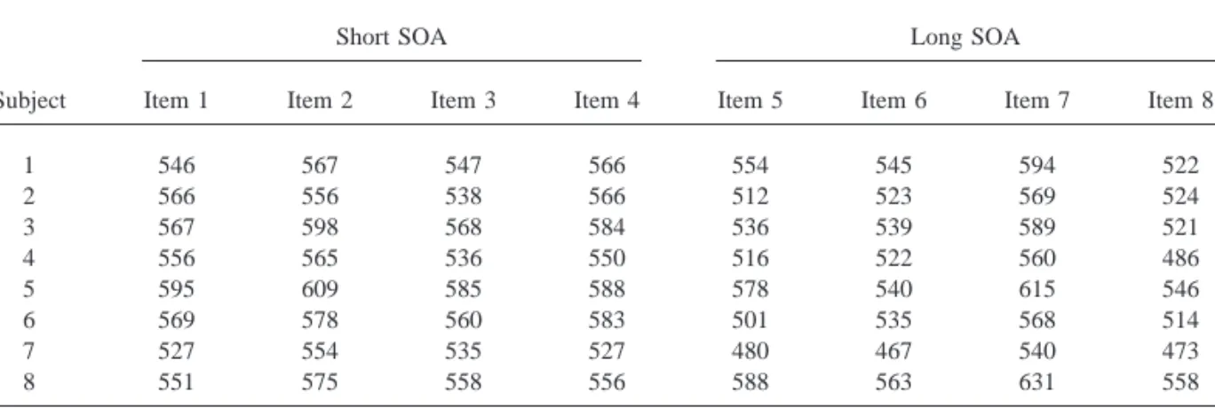
Table 2 gives a numerical example with sim-ulated data (example data have been included for most designs discussed in this article; the purpose of these examples is not to demonstrate a particular point but primarily to enable the interested reader to verify the results by carry-ing out the appropriate analyses uscarry-ing his/her favorite statistical package). In the present ex-ample, eight subjects are each tested under two conditions (a short and long SOA, respectively). There are eight items, four of which are
ran-domly assigned to each of the two conditions. The data were generated using a model in which there was no real effect of condition. Table 3 gives the ANOVA table corresponding to these data. Application of Eq. (2) gives F9(1,9)51.70. In practice, however, F9 will be difficult to compute due to missing data (e.g., error re-sponses) and limitations in the size of the ANOVA designs in most statistical packages (especially if a program based on the General Linear Model is used). It is then easier to com-pute its lower bound minF9, using the F values of separate subject and item analyses, usually referred to as F1 and F2, respectively. In a
subject analysis each data point in a cell of the
design is computed by collapsing over items, whereas in an item analysis data points are computed by collapsing over subjects. Although
minF9 is linked to an analysis that treats sub-jects and language materials (items) as random effects in a single ANOVA model, this statistic TABLE 2
Simulated Data for Repeated-Measurements ANOVA with Words Sampled Randomly
Subject
Short SOA Long SOA
Item 1 Item 2 Item 3 Item 4 Item 5 Item 6 Item 7 Item 8
1 546 567 547 566 554 545 594 522
2 566 556 538 566 512 523 569 524
3 567 598 568 584 536 539 589 521
4 556 565 536 550 516 522 560 486
5 595 609 585 588 578 540 615 546
6 569 578 560 583 501 535 568 514
7 527 554 535 527 480 467 540 473
8 551 575 558 556 588 563 631 558
TABLE 3
ANOVA Summary Table for Example Data for Table 2 Source of variation df Mean-square
Treatment 1 8032.6
Words (within Treatments) 6 3695.7
Subjects 7 3750.2
Treatment3Subjects 7 1083.8
can be computed by the F values from separate subject and item analyses. As shown by Clark (1973):
minF95 MSA MSAS1MSW(A)5
F1F2
F11F2
. [5]
For the data in Table 2, F1(1,7)5 7.41 and
F2(1,6)5 2.17, hence minF9(1,10) 5 1.68. It is evident that using F1 would lead to an incorrect conclusion. In this example, F2 does much better and minF9is actually quite close to
F9. These data reiterate the point made by Clark (1973) about the bias that would be present if F1 was used to test the difference between the conditions.
Clark’s paper was highly influential and it is now customary (especially among language re-searchers) to routinely run both an item and a subject analysis. But it appears that there has been some misconception with respect to the nature of the problem and the solution proposed by Clark (1973). Many researchers have been testing their treatment effects on the basis of separate subject and item analyses and have rejected the null hypothesis if both analyses showed significant F values. However, this pro-cedure, which will hereafter be denoted as the
F1 3 F2 criterion, is not equivalent to the
minF9 solution and leads to positive bias (a higherathan the nominala) if item variance is not controlled for, as a theoretical analysis shows and as Forster and Dickinson (1976) demonstrate by Monte Carlo simulations. Of course asserting a difference when either F1or
F2is significant would result in an even greater bias.
In this article we first review Clark’s solution and show that the F1 3 F2 criterion, although widely used, leads to positive bias. Next, we discuss alternatives to the minF9 approach and consider the effects of commonly used varia-tions in the exact nature of the design (such as matching of items and counterbalancing of lists) that affect the outcome of the analysis. We hope to convince the reader that it is necessary to take the details of the experimental design into
ac-count before deciding on the particular ANOVA to be performed.
CURRENT PRACTICE: THE F1 3 F2 FALLACY
Although there was some controversy in the late 1970s regarding the necessity and appropri-ateness of treating items as a random factor in the analysis of experiments with language ma-terials (see Cohen, 1976; Smith, 1976; Wike & Church, 1976; see also Clark, 1976), by the early 1980s the issue was more or less settled and researchers started to routinely perform both subject and item analyses. However, many researchers seem to believe that the subject analysis (F1) makes it possible to test for reli-ability of the effect over subjects and that the item analysis (F2) makes it possible to test for reliability of the effect over items. Hence, if both F statistics are significant, it should (ac-cording to this reasoning) be the case that the effect is reliable over both subjects and items.
However, this is incorrect since in the stan-dard design considered by Clark (1973) both F1 and F2 will be biased when subjects and items are sampled randomly. To see this, note that if
F1 and F2 are equal, F1 5 F2 5 F, hence
minF9 5F/ 2. Thus, both F1 and F2 could be significant, while minF9would not. If this hap-pens, many researchers seem to be hesitant to accept that the effect is not significant. An ex-ample may be found in Katz (1989, p. 492). After obtaining an F1of 10.8 and an F2of 5.44 (both p’s , .05), Katz reluctantly concludes: “The effect of concreteness was marginally sig-nificant when the overly conservative minF test was computed; minF(1,44) 5 3.62, p , .10.” Most researchers today do not even com-pute or report the value of minF9. In some cases a rather curious mixed approach is used. For example, Seidenberg et al. (1984, p. 386) report: “Min F9 statistics were calculated, and are reported when they were significant; other-wise, the significant F statistics for the subject and item analyses are reported.”
Sometimes this procedure is justified by the argument that the minF9 procedure is a too conservative test (see the quote above) and that this F13F2procedure avoids both this bias in
minF9 as well as the bias in F1. For example, Smith (1976) and Wike and Church (1976) crit-icized the use of F9 (and minF9) as being an unduly conservative test. The power of the test based on F9 depends on a number of factors such as the structure of F9 (the terms included in its calculation), the size of the error variance, the number of the degrees of freedom, and the number of levels of the treatment variable. However, Monte Carlo simulations with F9 as in Eq. (2) have demonstrated that it is a good approximation to the normal F statistic (Dav-enport & Webster, 1973; Forster & Dickinson, 1976). Furthermore, as Forster and Dickinson (1976) have shown, minF9is a good estimate of
F9, and both statistics are not unduly conserva-tive, given thatsW(A)2 andsAS2 , the variance com-ponents expressing item and subject variability, are not too small (relative to sW(A)S2 ). In most experiments this is likely to be the case.
In addition, Wike and Church (1976) com-mented that although F9 has an approximate F distribution, little is known about the character-istics of its distribution. In most psycholinguis-tic and semanpsycholinguis-tic memory tasks dependent vari-ables such as reaction times are not normally distributed. The conventional F test is robust against violations of homogeneity of variance and normality of the distribution of the depen-dent variable. However, Santa, Miller, and Shaw (1979) demonstrated that the F9 and
minF9are also robust against violations of ho-mogeneity and normality. They showed by means of Monte Carlo simulations that with heterogeneous treatment group variances and with five types of error distributions (normal, exponential, log-uniform, binary, and log-nor-mal) the F9 and minF9 have real alpha values that are near the nominal alpha value of .05. Only when the variance componentssW(A)2 and sAS2
are small do both statistics tend to be con-servative.
Thus, there is no justification for the assertion that the minF9 procedure advocated by Clark (1973) is too conservative. Hence, the argument that the F1 3 F2 procedure may be justified because of the conservative nature of minF9 is incorrect. Rather, the situation is the other way around. As Forster and Dickinson (1976) have
shown by means of Monte Carlo simulations, the F1 3 F2 procedure has a larger error rate than .05 although of course not as large as separate F1 or F2 analyses.
To give some indication of this “F1 3 F2 fallacy”, we screened Volumes 32–37 (1993– 1997) of the Journal of Memory and Language and counted how many of the published papers reported both F1 and F2 in at least one exper-iment. In these volumes there were a total of 220 papers, of which 120 reported F1 and F2 without mentioning any minF9 values. In only 4 papers were F1, F2, and minF9 values re-ported. Thus, these statistics clearly show that the F1 3 F2 fallacy is quite widespread.
2
Widespread as it may be, this fallacy did not become common practice immediately after the appearance of Clark’s paper. Initially, research-ers based their conclusions on the outcome of the minF9test and often did not even report the
F1 and F2 statistics. Today, the situation is completely the opposite. To demonstrate this, we first counted all papers between 1974 and 1997 of the Journal of Verbal Learning and
Verbal Behavior/Journal of Memory and Lan-guage that reported minF9 and/or F1 and F2 and then computed the proportion of those pa-pers that reported minF9and not just F1and F2. These proportions are plotted in Fig. 1. The results are clear: there is a steady change from a situation in which the F1 3 F2 criterion is never used to a situation in which the minF9 criterion is almost never used.
Of course, the conclusions that were based on the F1 3 F2 testing procedure in the screened papers need not be incorrect. As we show be-low, if the researchers experimentally con-trolled for item variability, the use of F1 by itself might have been the correct procedure. In that case, the use of F13 F2 would only have been a more conservative procedure and all significant results would remain significant (al-though some results that were reported as not
2
It is of some interest that the use of item analyses and minF9seems to be restricted to those analyses in which the dependent variable is reaction time, although from a statis-tical point of view there is no reason why the “language-as-fixed-effect” issue should not be relevant when accuracy measures are analyzed.
significant might in fact be significant). How-ever, if in these studies subjects and items were in fact sampled (quasi-)randomly the use of
minF9might have led to different conclusions. MATCHING OF ITEMS
Error variance introduced by random or pseu-dorandom selection of items can be controlled by statistical or experimental procedures. Sta-tistical control can be achieved by adding an item variance component to the ANOVA model, and hypothesis testing is then based on the computation of F9 or its lower bound
minF9. This was the solution proposed by Clark. Item variance can, however, also be con-trolled by experimental procedures such as matching stimulus materials in different treat-ment groups with respect to variables that cor-relate highly with the dependent variable. This seems to be the preferred approach in current research. It is rarely the case that investigators select their stimulus materials in a truly random fashion. Normally, items are carefully selected and balanced on important variables that corre-late with the response measure. Of course, if balancing is used to control item variance it will replace the requirement to control by statistical procedures, i.e., applying the random effect model (F9). In that case item variability would
not affect the differences between the treatment conditions and it would be best to perform a subject (F1) analysis, where subjects form the only random variable. Wickens and Keppel (1983) showed that if item variance is con-trolled in this manner, the bias in F1 is indeed greatly reduced. Moreover, if the blocking fac-tor is ignored in the analysis, it is best to per-form a F1 analysis because in that case the usage of F9 or minF9 leads to a considerable reduction in power (see Wickens & Keppel, 1983, p. 307). Of course, if it were possible to do the full analysis (including subjects as well as blocks), that would be the preferred analysis. However, as explained earlier, this is rarely possible.
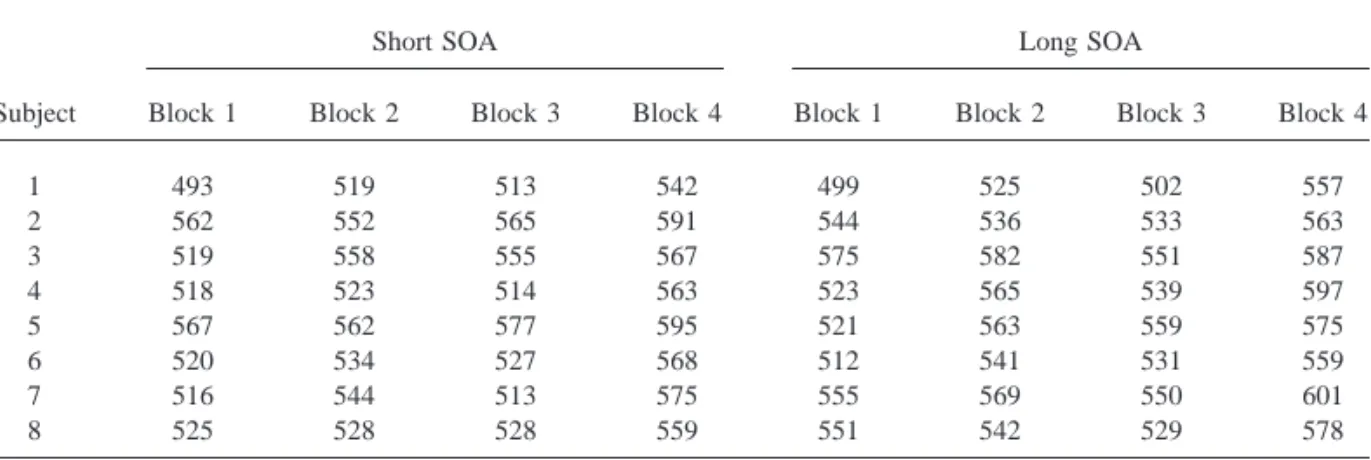
To illustrate these points, we will take a closer look at the ideal case in which this type of blocking or matching captures all of the system-atic variability between items. That is, the two (or more if there are more treatment conditions) items within a block are perfectly matched. The various blocks are still assumed to be sampled randomly from a larger population of blocks. The major difference in such a design is that the blocks factor will be crossed with treatments instead of being nested under treatments as was the case when items are randomly sampled. To make it easier to understand the nature of this design, we constructed a small set of simulated data in which there are again eight subjects, each tested under two conditions (see Table 4). Suppose that we are able to select pairs of items in such a way that they are matched on the most important item variables that affect the lexical decision times. Hence, there will be four pairs of matched items or blocks. Within each block, one item is assigned to each of the two experi-mental conditions. Note that both items of a given pair of matched items have been given the same block label in order to emphasize the blocking. The data were again generated using a model in which there was no real effect of condition.
Table 5 gives the expected mean-squares for such a design. This case is similar to the tradi-tional case in that here too there is no simple F statistic to test the significance of the treatment effect. A quasi-F ratio that may be used to
FIG. 1. The proportion of papers that report minF9of all papers that report F1and F2(based on a count of all papers in JVLVB/JML between 1974 and 1997). Data are grouped in 2-year intervals.
evaluate the significance of the treatment effect, is given by
F95MSA1MSABS MSAS1MSAB
. [6]
Wickens and Keppel (1983) showed that in such a design with blocking of materials, the bias in the F ratio from the standard subject analysis (F1) is greatly reduced. To see this more clearly, note that
E~F1!
[7] < E~MSA!
E~MSAS!
5se 2
1sABS 2
1qsAS 2
1nsAB 2
1nqsA 2
se
21s
ABS
2 1
qsAS
2 .
Hence the bias in F1 is now a function ofsAB 2
, the interaction between blocks and treatments, and this will usually be smaller thansW(A)2 , the variability of items within treatments that is responsible for the bias in the case where items are sampled randomly (i.e., not matched).
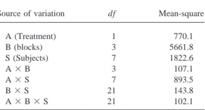
Table 6 gives the full ANOVA table corre-sponding to the example data of Table 4. Apply-ing Eq. (6) gives F9(1,8)5 0.87. For these data,
F1(1,7)50.86 and F2(1,3)57.19 (if the match-ing is taken into account, i.e., if a repeated-mea-sures design is used in the item analysis, as would be appropriate), hence minF9(1,3)5 0.77. If the matching is not taken into account, F2(1,6) 5 0.27, hence minF9(1,10)50.20. It is evident that if the matching is taken into account both minF9 and F1give a good approximation to the “true” F9. If the matching is not taken into account, F2 is quite a bit smaller and minF9underestimates the TABLE 4
Simulated Data for Repeated-Measurements ANOVA with Matched Items
Subject
Short SOA Long SOA
Block 1 Block 2 Block 3 Block 4 Block 1 Block 2 Block 3 Block 4
1 493 519 513 542 499 525 502 557
2 562 552 565 591 544 536 533 563
3 519 558 555 567 575 582 551 587
4 518 523 514 563 523 565 539 597
5 567 562 577 595 521 563 559 575
6 520 534 527 568 512 541 531 559
7 516 544 513 575 555 569 550 601
8 525 528 528 559 551 542 529 578
TABLE 5
Expected Mean-Squares for Repeated-Measurements ANOVA with Blocks or Matched Items Crossed with Treatments
Source of variation df Expected mean-squares
A (Treatment) p 21 se
2
1sABS 2
1qsAS 2
1nsAB 2
1nqsA 2
B (blocks) q 21 se
2
1psBS 2
1npsB 2
S (Subjects) n 21 se
2
1psBS 2
1pqsS 2
A3B (p21)(q2 1) se
2
1sABS 2
1nsAB 2
A3S (p21)(n2 1) se
2
1sABS 2
1qsAS 2
B3S (q21)(n2 1) se
2
1psBS 2
A3B3S (p21)(q2 1)(n21) se
2
1sABS 2
Note. p5number of levels of the treatment variable; n5number of subjects; q5 number of blocks. Blocks and Subjects are assumed to be random effects.
correct value of F9. As we mentioned before, Wickens and Keppel (1983) showed that this is a general finding in this type of design. Thus, if it is not possible (because of missing data) to do the full analysis that includes the blocking factor (leading to F9), it is better to simply use F1rather than minF9, especially when the matching of the items is not taken into account in the item analysis used to determine F2.
COUNTERBALANCED DESIGNS In many cases, however, better ways of con-trolling item variability are possible. One such approach involves the case where items are sampled randomly for each subject separately. In this case each subject receives a different set of words under each of the treatment levels. This case was briefly mentioned by Clark (1973, p. 348) as one where the traditional anal-ysis (F1) is correct (see also Winer, 1971, p. 365). In such a design where Items are nested within Subjects and Treatments, the treatment effect may be tested against the Treatment 3 Subjects interaction, which is equivalent to the regular F1test when the data are collapsed over items.
An alternative approach that is frequently used in memory research is the use of counter-balanced lists. In such a design, one group of subjects receives List 1 in condition 1 and List 2 in condition 2, and a second group of subjects receives List 2 in condition 1 and List 1 in condition 2. In this design, the between-groups variability is confounded with (part of) the in-teraction between list and treatment. However, and this is of course the rationale for using such
a design, the mean difference between the treat-ment conditions (and hence the treattreat-ment effect) is not affected by any difference that might exist between the lists.
Table 7 gives a numerical example with three experimental conditions and three lists of four items each. Hence there are three groups of subjects and the assignment of lists to condi-tions is counterbalanced across groups. As be-fore, it is normally not possible to analyze such a complete design and the experimenter will have to average the scores for the four items within each condition. These averages are given in Table 8. How should such data be analyzed, taking into account that the factor Lists should be a random effect?
In order to answer this question, we will take a closer look at the expected mean-squares for this design (see Table 9). This type of design is discussed by Winer (1971, pp. 712, 716) and Kirk (1982, p. 648), although they treated the factor corresponding to Lists as fixed. Kirk re-fers to this design as a Latin Square Confounded Factorial design (LSCF). The ANOVA model for this design is as follows:
Xijm(t)5m 1 ut1pm(t)1ai
1bj1ab9ij1eijm(t),
[8]
wherem5overall mean;ut5effect of group t (5the between-component of the Treatment3 List interaction); pm(t) 5 effect of subject m (nested within group t),ai 5 effect of the ex-perimental treatment i; bj 5 effect of list j; ab9ij 5 the within-component of the Treat-ment3List interaction; andeijm(t)5 experimen-tal error (a residual term equivalent to the in-teraction between Treatment, List, and Subjects plus “real” error; this term might be further decomposed but this would not affect the re-sults). Due to the nature of this design (each group receives only p of the p 3 p
combina-tions of Treatment and List), the interaction between Treatment and List is divided into two components, one between subjects and one within subjects.
In the ANOVA model it is assumed that Group, Subjects within Groups, as well as List TABLE 6
ANOVA Summary Table for Example Data of Table 4 Source of variation df Mean-square
A (Treatment) 1 770.1
B (blocks) 3 5661.8
S (Subjects) 7 1822.6
A3B 3 107.1
A3S 7 893.5
B3S 21 143.8
are random factors (Group is random since it corresponds to an interaction between a fixed and a random effect). That is, it is assumed that the lists are based on a random sample of words from a larger population of words. Table 9 gives the expected mean-squares for this design under these assumptions. Note that the interaction term Treatment3 List (within) does not exist for the case p 5 2 (this interaction is then completely confounded with the Group main effect).
As can be seen from Table 9, in order to test the treatment effect, the treatment mean-square should be tested against the Treatment3 List (within) mean-square. If the F test for the Treat-ment 3 List (within) interaction effect is not significant by a conservative criterion (a5.25), this mean-square may be pooled with the error (residual) mean-square, giving a much more powerful test for the treatment effect. In the special case where p 5 2, the treatment effect is always tested against the error mean-square. Hence, in all of these cases there is no necessity to run two analyses, one over subjects and one over items. The subject analysis (i.e., the
anal-ysis in which all items from a single list are averaged) will give all the information that is required to test the significance of the treatment effect. Moreover, there is no necessity to com-pute a quasi-F ratio: regular F-ratios will be correct.
This design was also discussed by Pollatsek and Well (1995, Table 4), except that they de-noted the main effect of List as the Groups 3 Treatment interaction. However, as mentioned above, these two effects are equivalent in the
p5 2 case. In the case p . 2, the Groups3 Treatment interaction consists of two terms, namely the main effect of List and the within-part of the Treatment 3 List interaction. In order to separate these effects, two ANOVA’s should be run, the traditional one without the List effect but with the Groups 3 Treatment interaction and a second one with the List effect but without the Groups 3 Treatment interac-tion. The latter analysis gives the correct value for the List sums-of-squares, and subtracting this from the sums-of-squares for the Groups3 Treatment interaction gives the correct value for the within-part of the Treatment3List interac-TABLE 7
Simulated Data for Design Using Counterbalanced Lists
Group Subject
Short SOA Medium SOA Long SOA
Item 1 Item 2 Item 3 Item 4 Item 5 Item 6 Item 7 Item 8 Item 9 Item 10 Item 11 Item 12
1 1 532 508 522 482 468 496 544 547 475 522 502 484
2 542 516 545 483 509 519 588 583 499 535 535 486
3 615 584 595 560 542 591 630 617 543 606 560 545
4 547 553 584 535 514 555 591 606 538 565 546 527
Item 9 Item 10 Item 11 Item 12 Item 1 Item 2 Item 3 Item 4 Item 5 Item 6 Item 7 Item 8
2 5 553 598 581 551 619 576 606 561 548 590 614 631
6 464 502 485 451 484 479 499 471 447 486 514 523
7 481 511 492 472 531 506 542 475 471 510 539 556
8 541 588 551 533 582 556 589 515 538 545 601 576
Item 5 Item 6 Item 7 Item 8 Item 9 Item 10 Item 11 Item 12 Item 1 Item 2 Item 3 Item 4
3 9 482 530 571 563 501 561 500 506 543 539 558 497
10 559 570 632 639 551 592 572 561 617 587 616 549
11 462 497 546 538 487 546 491 470 529 508 525 473
tion. This partitioning of the Groups 3 Treat-ment interaction was also briefly discussed by Pollatsek and Well (1995, Appendix A, espe-cially Table A2), although the expected mean-squares that they present apply to the case that the List factor is assumed fixed rather than random. Contrary to the suggestion of Pollatsek and Well (1995), however, it is not required to do separate analyses over subjects and items in order to test the effect of the treatment factor. The expected mean-squares, under the assump-tion that List is a random effect, show that the
Treatment effect can always be tested directly using the mean-squares obtained from the stan-dard subject analysis (averaging over items).
In Table 10 we present the ANOVA sum-mary table for the data presented in Table 8. As explained above, the Treatment 3 List Sums-of-Squares was obtained by subtracting the List main effect Sums-of-Squares (3106.2) from the Group3Treatment Sums-of-Squares (3152.3). If we test the Treatment main effect against the Treatment 3 Lists interaction, the resulting F ratio equals F(2,2) 5 1.116. However, since the Treatment3Lists interaction is not signif-icant [F(2,18)50.786], a more powerful test may be obtained by pooling this interaction and the error Sums-of-Squares and testing the treat-ment effect against this pooled error. Note that this pooled error Sums-of-Squares may be ob-tained directly from the analysis that includes the List main effect but not the Group3 Treat-ment interaction effect. This gives an error term for the F test that is based on 20 degrees of freedom instead of just 2. In the present exam-ple, the resulting F value is 0.896.
CONCLUSION
There are two important conclusions that we draw from these analyses. The first is that many language researchers are applying statistical procedures that do not match the details of the actual design that they are using. In many cases the design does not require separate analyses over subjects and items, yet such analyses are routinely run, without taking into account that this procedure was originally introduced for a TABLE 8
Data from Table 7 Collapsed over Items
Group Subject
Short SOA List 1
Medium SOA List 2
Long SOA List 3
1 1 511 514 496
2 522 550 514
3 588 595 563
4 554 567 544
List 3 List 1 List 2
2 5 571 591 596
6 476 483 492
7 489 514 519
8 553 560 565
List 2 List 3 List 1
3 9 536 517 534
10 600 569 592
11 511 498 509
12 490 476 483
TABLE 9
Expected Mean-Squares for Repeated-Measurements ANOVA with Counterbalanced Lists
Source of variation df Expected mean-squares
G (groups) (5A3L between) p21 se
21ps S(G) 2 1nps
G 2
S(G) p(n21) se
21ps S(G) 2
A p21 se
21ns AL 2 1nps
A 2
L (lists) p21 se
21nps L 2
A3L (within) (p2 1)(p22) se
21ns AL 2
Residual p(n21)(p21) se
2
Note. p5number of groups5number of levels of the treatment variable5number of lists; n5number of subjects within each group. Lists and Subjects are assumed to be random effects.
very specific design, namely a design where the items are nested under the treatment variable. If this is not in fact the case, e.g., when the mate-rials have been matched on a number of vari-ables or when the lists are counterbalanced over different groups of subjects, there is no need to compute (min) F9and the simple subject anal-ysis (averaging over items) will be correct. The second conclusion is that the practice of running both a subject and an item analysis and of using the F1 3 F2 criterion is both widespread as well as without any foundation. Either F1 is correct or it is incorrect. In the latter case, (min)
F9 is the correct statistic to compute. REFERENCES
Clark, H. H. (1973). The language-as-fixed-effect fallacy: A critique of language statistics in psychological re-search. Journal of Verbal Learning and Verbal Behav-ior, 12, 335–359.
Clark, H. H. (1976). Reply to Wike and Church. Journal of Verbal Learning and Verbal Behavior, 15, 257–261. Cohen, J. (1976). Random means random. Journal of
Ver-bal Learning and VerVer-bal Behavior, 15, 261–262. Coleman, E. B. (1964). Generalizing to a language
popula-tion. Psychological Reports, 14, 219 –226.
Davenport, J. M., & Webster, J. T. (1973). A comparison of some approximate F-tests. Technometrics, 15, 779 – 789.
Forster, K. I., & Dickinson, R. G. (1976). More on the language-as-fixed-effect fallacy: Monte Carlo esti-mates of error rates for F1, F2, F9, and minF9.
Jour-nal of Verbal Learning and Verbal Behavior, 15, 135– 142.
Katz, A. N. (1989). On choosing the vehicles of metaphors: Referential concreteness, semantic distances, and indi-vidual differences. Journal of Memory and Language, 28, 486 – 499.
Kirk, R. E. (1982). Experimental design: procedures for the behavioral sciences. Pacific Grove: Brooks/Cole. Pollatsek, A., & Well, A. D. (1995). On the use of
coun-terbalanced designs in cognitive research: A sugges-tion for a better and more powerful analysis. Journal of Experimental Psychology: Learning, Memory, and Cognition, 21, 785–794.
Santa, J. L., Miller, J. J., & Shaw, M. L. (1979). Using quasi F to prevent alpha inflation due to stimulus variation. Psychological Bulletin, 86, 37– 46.
Seidenberg, M. S., Waters, G. S., Barnes, M. A., & Tan-nenhaus, M. K. (1984). When does irregular spelling or pronunciation influence word recognition? Journal of Verbal Learning and Verbal Behavior, 23, 383– 404. Smith, J. E. K. (1976). The assuming-will-make-it-so
fal-lacy. Journal of Verbal Learning and Verbal Behavior, 15, 262–263.
Wickens, T. D., & Keppel, G. (1983). On the choice of design and of test statistic in the analysis of experi-ments with sampled materials. Journal of Verbal Learning and Verbal Behavior, 22, 296 –309. Wike, E. L., & Church, J. D. (1976). Comments on Clark’s
“The language-as-fixed-effect fallacy.” Journal of Ver-bal Learning and VerVer-bal Behavior, 15, 249 –255. Winer, B. J. (1971). Statistical principles in experimental
design. New York: McGraw–Hill. (Received September 22, 1997) (Revision received February 19, 1999) TABLE 10
ANOVA Summary Table for Example Data of Table 8
Source of variation SS df MS F
G (groups) (5A3L between) 1720.2 2 860.08 0.164
S(G) 47206.2 9 5245.13 178.527
A 51.5 2 25.75 1.116
L (lists) 3106.2 2 1553.08 52.862
A3L (within) 46.2 2 23.08 0.786
Error 528.8 18 29.38