Multiple Imputation for Missing Data
in Repeated Measurements Using MCMC and
Copulas
Lily Ingsrisawang and Duangporn Potawee
Abstract— This paper presents two imputation methods: Markov Chain Monte Carlo (MCMC) and Copulas to handle missing data in repeated measurements. Simulation studies were performed using the Monte Carlo technique to generate datasets in different situations. Each subject unit in each dataset was measured on three occasions under the following conditions: 1. data had a multivariate normal distribution under two types of correlation structures: Compound Symmetry (CS) and Autoregressive (AR (1)), 2. the correlation among repeated observations under each subject was determined at low level (
ρ
=0.3), middle level (ρ
=0.5), and high level (ρ
=0.7), 3. sample sizes consisted of 30, 70, and 100 subject units, and 4. data were assigned missing at random (MAR) at the last occasion of measurement with missing rate of 5%, 10%, 20% and 30%, respectively. All possible combinations of these conditions gave rise a total of 72 different situations. Each defined situation was repeated 1,000 times by SAS programming and each missing value was replaced with a set of five plausible values that represent the uncertainty about the right value to impute under the MCMC method. The performance of each imputation method was evaluated using mean square error (MSE). The lower MSE would indicate the more effective method. The results from the simulation studies showed that the Copulas method was superior effective than other methods in all situations. The MCMC method was more effective than the simple mean imputation method when the correlation structure was AR1. For application, both imputation methods were applied with two datasets in practices: 1) waist circumference data on healthy project and 2) monthly rainfall data. The results also confirmed that the Copulas was the most effective method which was consistent with the simulation studies.Index Terms— Markov Chain Monte Carlo, Copulas, missing at random, repeated measuremens.
I. INTRODUCTION
N
repeated measures data analysis, it often faces with the problem of incomplete data when a subject has one or more missing values during the subsequent waves of data collection. The occurrence of missing values may due to any causes related to a study unit such as nonresponse, refusal, drop out, lost of follow up, illness or death. In theManuscript received January 16, 2012.
L. Ingsrisawang is with Department of Statistics, Faculty of Science, Kasetsart University, Bangkok, Thailand (corresponding author: phone number: +66 2 5625555 EXT 4514; fax: +66 2 9428384; email:
D. Potawee is with Department of Statistics, Faculty of Science, Kasetsart University, Bangkok, Thailand (email: [email protected])
meantime, missing values can be generated from human errors on either forget to ask a question or forget to record the answer. The patterns of missing data may be one of these special patterns: 1) univariate missing data, 2) unit nonresponse, or 3) monotone missing data. Firstly, the “univariate” missing data are restricted to missing values on a single variable while the other variables are fully recorded. Secondly, the “unit nonresponse” missing data have missing values on a block of variables for the same set of cases, and the rest of variables are all complete. Thirdly, the “monotone” missing data have the pattern of missing values after all variables are arranged such that
X ,X ,…,X :
1 2 j1, 2, ,
1; >1
=
…
−
j
k
k
X
j1
X
j+, then the variable will be observed whenever the variable is observed [8], [12]. To handle problems of missing data, one simplest approach is to focus on a complete-case analysis, but its disadvantage is the decreasing on statistical power from the smaller sample size [9], [10]. Another approach for analyzing incomplete data is using imputation methods to impute the best estimate of a missing value of the variable [7], [12]. Imputation methods base on three types of missingness as follows: 1) missing completely at random (MCAR, if the missingness is independent of both unobserved and observed data), 2) missing at random (MAR, if the missingness depends on observed data, but not on unobserved data), and 3) missing not at random (MNAR, if the missingness depends on unobserved data) [7], [13]. Multiple imputation (MI), under imputation approach, is proposed by Rubin [2] to analyze incomplete data under MAR mechanism. The idea of MI procedure is to replace each missing value with a set of M possible values. These values are drawn from the distribution of the study data under the uncertainty about the right value to impute. Then, analyze the imputed data sets from standard procedure for complete data and combine the results from these analyses [1], [13]. According to the MI concepts, this study aims to 1) present the possibilities of using two imputation methods: Markov Chain Monte Carlo (MCMC) and Copulas to impute the best estimates of missing values under MAR mechanism in repeated measurements, and 2) compare the performance of the MCMC and Copulas methods in estimating the missing values.
II. METHODS
A. Generating Datasets with Missing Values
A number of complete datasets were generated to have data on all three repeated measurements. Let
Y ,Y ,
1 2 and3
Y
be three continuous variables for three measurements on each subject at time point 1, 2, and 3, respectively. Under the assumption of a multivariate normal distribution with zero mean vector and variance-covariance matrix∑
,,
11 12 13
21 22 23
∑ =
⎡
σ
σ
σ
⎤
⎢
σ
σ
σ
⎥
⎢
⎥
⎢
σ
31σ
32σ
33⎥
⎣
⎦
⎣
⎦
1 2
Y ,Y ,
C S =
and are correlated under two types of
correlation structures, including compound symmetry (CS):
3
Y
R
1
ρ
ρ
1
1
⎡
ρ
ρ
⎤
⎢
ρ
ρ
⎥
⎢
⎥
⎢
⎥
and first order autoregressive (AR(1)) :
, 2
AR (1 ) 2
1
R
1
1
=
⎡
ρ ρ
⎤
⎢
⎥
ρ
ρ
⎢
⎥
⎢
ρ
ρ
⎥
⎣
⎦
where ij
ij
; i, j = 1, 2, 3.
σ
ρ =
σ
iiσ
jj3 3 3 72
× × × =
i 0 0 1 1 i 1 i 1 i i 1 i 1
P[X x | X
x ,X x , ,X
x ]
P[X x | X
x ].
− −
− −
The correlation among repeated observations under each subject was determined at low level (ρ =0.3), middle level (ρ =0.5), and high level (ρ=0.7). Sample sizes considered were 30, 70, and 100 subject units. Additionally, data were assumed MAR at the last occasion of measurement, ,
with missing rate of 5%, 10%, 20% and 30%, respectively. All possible combinations of these conditions gave rise a total of
2
different situations for 72 different datasets.3
Y
B. Imputation Methods
In each dataset, a simple imputation method was used to replace the missing value with a single value of the variable’s mean of the complete cases. This single imputation did not reflect the uncertainty about the prediction of the unknown missing values. Then, two advanced imputation methods, MCMC and Copulas, were used to estimate the missing value under MAR mechanism in repeated measures
.
C. MCMC
MCMC is a numerical method for generating pseudo-random drawn from probability distributions via Markov Chains. A Markov chain is a sequence of random variables
element given all previous ones depends only on the most recent value, i.e. for all i ,
<
=
=
=
=
<
=
…
A chain of random variables must be created long enough to approach to the approximate stationary distribution. By repeated simulation steps of the chain, one simulates draws samples from the stationary distribution [1], [7].
Reference [7]
suggested using MCMC to impute missing values by assuming: 1) data is from a multivariate normal distribution, 2) data are MCAR or MAR, and 3) the missing data pattern can be either monotone or arbitrary. To begin the MCMC process, a vector of means (μ)
and a variance-covariance matrix (Σ)
from the complete data (or available cases) are computed and used as the initial estimates for the Expectation-Maximization (EM) algorithm. The resulting EM estimates are used to be the starting values to estimate the parameters of the prior distributions for means and variances of the multivariate normal distribution with informative prior. In MCMC, the imputation step (I-step) simulates values of missing items by randomly selecting a value from the conditional distribution of missing values, , given the observed values, . Next, the posterior step (P-step) updates the posterior distribution of the mean and covariance parameters (e.g., normal distribution for the means and inverted Wishart distribution for covariance matrix [3]). Then, the vector of means and covariance matrix are simulated from the posterior distribution based on the updated parameters. The new estimates will be used in the I-step. Both the I-step and the P-step are iterated until the mean vector and covariance matrix are unchanged. The imputation from the final iteration will be used to form a complete data set.) miss ( i
Y
Y
i(obs)This study applied the MCMC method with the predetermined 72 different situations of repeated measurements. Each defined situation was repeated 1,000 times by using SAS procedures and each missing value was replaced with a set of five plausible values from posterior predictive distribution that represent the uncertainty about the right value to impute. Finally, the results from the five plausible values of each missing value were combined and used their average value to be the best estimates of each missing value.
D. Copulas
where
F is the distribution function on
ℜ
k
F ,F , ,F
1 2…
nare univariate marginal distributions, is a multivariate distribution function with marginals ,1 1 2 2 n n
C(F (x ),F (x ), ,F (x ))
…
1 2 n
F ,F , ,F
…
and C is copula function.
If one knows the joint distribution of
X
=
a vector of random variables, then one can impute the missing value from a conditional distribution of , a vector with missing values, given1 2 k
X X
X
( , , , )
…
k
X
,
H
=
which is a vector with complete data in history. 1 2 k
X X
X
( , , ,
…
−1)
)),
In this study, we applied the Gaussian copula in which the k-variate Gaussian copula with k Gaussian marginals corresponds to the k-variate Gaussian distribution. That is the multivariate normal distribution has normal marginal distributions and Gaussian copula dependence. Gaussian copula handles the dependence among univariate marginal distributions via the correlation matrix R of pairwise dependencies between variables. The multivariate Gaussian copula is defined as:
1 1 1
( (u ) , (u ) ,..., (u
k 1 1 1 2 1 k
C (u ,u ,...,u ;R)
k 1 2
k
=
Φ Φ− Φ− Φ−j
u (0,1)
∈
Φ
kj
X
j
F
Y
j-1 1
Φ
j j j
Y
=
[F (X )]
,
-1 1
Φ
where , j = 1, 2,…,k ; is the standard k variate normal distribution function with the correlation matrix R. For modeling the repeated measurements using The multivariate Gaussian copula, let have a continuous distribution function , j = 1,2, … , k, and let be its
normalizing transformation as where
is the inverse of the standard univariate Gaussian distribution function. Then, the joint multivariate distribution function is:
1 2 k k 1 2 k
F(y ,y ,... ,y ;R) C (u ,u ,...,u ;R)
=
=
1 1 1
k[ 1(u ),1 1 (u ),...,2 1 (u ); Rk
]
− − −
Φ Φ Φ Φ . (2) Then, we can find the MLE of missing value from the conditional distribution of . Lastly, the missing value ( ) can be replaced by:
k
y
k
f(y |H ,R)
k
y
k 1 CS
k
j 1
ˆy
1 (k 2)
=y ;
jρ
=
+ − ρ
∑
−
if R is under CS structure,
and ; if R is under
AR1 structure, where and are standard deviation at the (k-1)th and the kth occasion of measurement [5], [6].
k 1 k 1 k 1 k
k AR
k
(
y
Y
)
Y
S
S
yˆ
=
ρ
−−
−+
−
k 1
S
−S
kE. Comparison of Imputation Methods
Once the MCMC method has been implemented, it is necessary to check the convergence of the simulated sequence of random variables to the stationary distribution. However, it is not too difficult to apply the MCMC method for multiple imputations of missing values because it has commands available on some statistical packages such as PROC MI and PROC MINIMIZE in SAS program [1], [13]. In opposite, the copulas method is easy for computation but it is not easy to replace the values of missing data when there are lots of missing items. In addition, the data on repeated measurements those are prior to the observation of missing value must be complete. It also needs to check whether the correlation structure among repeated observations is under CS or AR(1). The performance of each imputation method can be evaluated from its value of mean square error (MSE). The lower MSE would indicate the more effective method [10].
III. RESULTS
To meet the objectives of study, we compared among three imputation methods: simple mean, MCMC and Copulasfor the best estimates of missing values under MAR mechanism in repeated measurements both in simulation and application of two real datasets.
A. Simulation Study
Table 1 and Table 2 showed the estimated MSE from simulation studies in 72 situations which are under different types of correlation structure, levels of correlation among repeated measurements, missing rates (%) at last measurement, and sample sizes. Results indicated that the Copulas method was the most effective in all situations. The MCMC method was more effective than the simple mean imputation method when the correlation structure was AR(1).
B. Application of Two Datasetss
We applied the MCMC and the Copulas algorithms for imputation of missing values in two real datasets with different correlation structure among repeated observations.
Dataset 1: The waist circumference data
The first dataset was obtained from a study on “healthy project” of the “Nopparat Rajathanee” hospital in Bangkok where the outcome of interest was waist circumference of each individual. The waist circumference data, including weight and height, were collected from participants on a monthly basis between November 2008 and February 2009. At least 105 participants have waist circumference values more than 80 and 90 centimeters and 44 participants were completely followed up for four months. The correlation among repeated observations of waist circumference under each subject was assigned at high level (ρ ) from the assuming CS correlation structure as data evidence-based shown in the below:
0.91625 0.9
⎤
⎥
⎥
⎥
⎥
⎦
CS
1
0.93662 0.92046 0.85249
0.93662
1
0.94599 0.83225
0.92046 0.94599
1
0.91625
0.85249 0.83225 0.91625
1
R
⎡
⎢
⎢
=
⎢
⎢
⎣
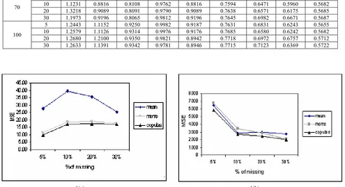
The data on the last occasion of measurements were assigned missing at random with missing rate of 5%, 10%, 20% and 30%, respectively. Next, we tested for the normal distribution of the waist circumference data containing missing values, checked for convergence of mean vector and covariance matrix under the MCMC process for MI, and compared the performance of three imputation methods: simple mean, MCMC, and Copulas. The result of study
showed that the MSE of the Copulas method is smallest at all level of missing rate (Fig. 1(a).) when compares with those of other imputation methods. For this dataset, the Copulas shows the most effective method for data imputation under CS correlation structure.
Dataset 2: The monthly rainfall data
The second dataset was from routine work of Thai Meteorological Department (TMD) where the outcomes of interest are the average of monthly rainfall in the northern region of Thailand. The data were collected from 28 local weather stations from June to August, 2009. The correlation among repeated observations of the average of monthly rainfall at each weather station was assigned at middle level ( ) from the assuming AR(1) correlation structure as data evidence-based shown in the below:
0.452 0.5
ρ= ≈
AR(1)
1
0.3566 0.189
R
0.3566
1
0.452
0.189 0.452
1
⎡
⎤
⎢
⎥
=⎢
⎥
⎢
⎥
⎣
⎦
The data on the average rain volume in August 2009 were assigned missing at random with missing rate of 5%, 10%, 20% and 30%, respectively. Next, we tested for the normal distribution of the average of monthly rainfall data which included missing values, checked for convergence of mean vector and covariance matrix under the MCMC process for MI, and compared the performance of the three imputation methods: simple mean, MCMC, and Copulas. The result of
study showed that the MSE of the Copulas method is smallest at all level of missing rates (Fig. 1(b).) when compares with other imputation methods. For this dataset, the Copulas also shows the most effective method for data imputation under AR(1) structure.
IV. DISCUSSION
Although the results from simulation studies indicated that the Copulas method was superior to the MCMC and the simple mean imputation methods, its performance depended on these factors, including missing rate (%) and level of correlation among repeated observations. If the sample size was fixed and the missing rate increased from 20% to 30%, there were much more difference in the values of MSE
both the Copulas and the MCMC method under missing rate 20% or 30% were closer in values. That is the performance of both imputation methods are almost equivalence when the level of missing rate was increased and the sample size is 70 or larger. Moreover, we found that the MSE values from all imputation methods of the simple mean, the MCMC and the Copulas would decrease when the level of correlation among repeated observations was increased under the condition of fixed sample size and fixed level of missing rate. In sum, the performance of the simple mean and the Copulas methods were higher than the MCMC when the level of correlation among repeated observations was increased under the CS structure. The MCMC and the Copulas gave better performance than the simple mean method under AR(1) structure when the level of correlation among repeated observations was increased.
V. CONCLUSION
The results from the simulation studies showed that the Copulas method was the most effective in all situations. The MCMC method was more effective than the simple mean imputation method when the correlation structure was under AR(1). For application, both imputation methods were applied with two datasets in practices: 1) waist circumference data on healthy project and 2) monthly rainfall data.
ACKNOWLEDGMENT
The authors thank the Nopparat Rajathanee hospital and the Thai Meteorological Department (TMD) as well as many individuals including the director of the hospital and the director and the officers of the TMD for sharing information and supporting data for this study.
REFERENCES
[1] A. Dmitrienko, G. Molenberghs, C. Chuang-Stein, and W. Offen,
Analysis of Clinical Trials Using SAS. NC: SAS Institute Inc. Cary,
2005.
[2] D.B. Rubin, Multiple Imputation for Nonresponse inSurveys. New
York: John Wiley & Sons, Inc., 1987.
[3] D.B. Rubin, “Multiple imputation after 18+ years,” Journal of the American Statistical Association, 91, 1996, pp. 473–489.
[4] D.F. Morrison, Multivariate Statistical Methods. The Wharton School
University of Pennsylvania, 2005.
[5] E. Kaarik, “Imputation algorithm using Copulas,” Metodoloski ki zvezki, 3(1), 2006, pp.109–120.
[6] E. Kaarik, “Imputation Modelling Dropouts by Conditional Distribution, a Copula-Based Approach. Institute of Mathematical
Statistical, University of Tartu, 2007.
[7] J.L. Schafer, Analysis of Incomplete Multivariate Data. London:
Chapman and Hall, Inc., 1997.
[8] J. Schafer, Missing Data in Longitudinal Studies: A Review.
Department of Statistics and the Methodology Center University of Pennsylvania, 2005.
[9] P.L. Roth, “Missing data: a conceptual review for applied psychologists,” Personnel Psychology., 47, 1994, pp. 537–559.
[10] R. Huang, and K.C. Carriere, “Comparison of methods for incomplete repeated measure data analysis in small sample,” Journal of Statistical
Planning and Inference, 136, 2006, pp. 235–247.
[11] R.B. Nelson, An Introduction to Copula. Lectures Notes in Statistic,
139, New York: Springer Verlag, 1999.
Table 1
Comparison of MSE among three imputation methods (simple mean, MCMC, and Copulas) from the simulation study under CS correlationstructure, level of correlation among repeated measurement (
ρ
), missing rate of last measurement (% ) and sample sizeMSE
ρ
= 0.3ρ
= 0.5ρ
= 0.7 Samplesize
missing rate
(%) Mean MCMC Copulas Mean MCMC Copulas Mean MCMC Copulas 5 1.0250 1.0171 0.8985 0.6712 0.7434 0.6539 0.5321 0.6773 0.4351 10 1.0240 1.0229 0.8536 0.7347 0.7782 0.6610 0.5431 0.5790 0.4436 20 1.0421 1.0440 0.8595 0.7221 0.8705 0.6724 0.5512 0.5494 0.4492 30
30 1.0500 1.1163 0.8561 0.7591 0.8942 0.6493 0.5578 0.5673 0.4343 5 1.0399 1.0536 0.8298 0.7386 0.8930 0.6587 0.4631 0.5678 0.4399 10 1.0449 1.0620 0.8417 0.7783 0.8977 0.6583 0.4849 0.5679 0.4403 20 1.0872 1.0643 0.8484 0.7646 0.8427 0.6612 0.4690 0.5355 0.4418 70
30 1.0295 1.0137 0.8518 0.7581 0.7869 0.6830 0.4920 0.5008 0.4642 5 1.0399 1.0079 0.8636 0.8515 0.8882 0.6796 0.5703 0.5663 0.4516 10 1.0210 1.0620 0.8648 0.8223 0.8270 0.6760 0.5349 0.5273 0.4494 20 1.0584 1.1036 0.8668 0.7874 0.8703 0.6722 0.4923 0.6480 0.4473 100
[image:5.595.48.543.378.647.2]30 1.0558 1.0751 0.8638 0.7770 0.8383 0.6717 0.4806 0.5326 0.4473
Table 2
Comparison of MSE among three imputation methods (simple mean, MCMC, and Copulas) from the simulation study under AR(1) correlationstructure, level of correlation among repeated measurement (
ρ
), missing rate of last measurement (% ) and sample sizeMSE
ρ
= 0.3ρ
= 0.5ρ
= 0.7 Samplesize
missing rate
(%) Mean MCMC Copulas Mean MCMC Copulas Mean MCMC Copulas 5 1.2283 1.1165 0.9350 1.2283 0.9196 0.7777 0.6394 0.6253 0.5367 10 1.4438 1.0514 0.9220 1.2251 0.8479 0.7643 0.6417 0.5736 0.5268 20 1.2449 1.1752 0.9342 0.9884 0.9110 0.7776 0.6525 0.6451 0.5393 30
30 1.2571 1.2290 0.9667 0.9974 0.9448 0.8049 0.6972 0.6860 0.5600 5 1.2321 0.9474 0.8125 0.9805 0.8544 0.7651 0.6983 0.6149 0.5698 10 1.1231 0.8816 0.8108 0.9762 0.8816 0.7594 0.6471 0.5960 0.5682 20 1.3218 0.9089 0.8091 0.9790 0.9089 0.7638 0.6571 0.6175 0.5685 70
30 1.1973 0.9196 0.8065 0.9812 0.9196 0.7645 0.6982 0.6671 0.5687 5 1.2443 1.1152 0.9250 0.9982 0.9187 0.7631 0.6831 0.6243 0.5655 10 1.2579 1.1126 0.9314 0.9976 0.9176 0.7685 0.6580 0.6242 0.5682 20 1.2680 1.2100 0.9350 0.9821 0.8942 0.7718 0.6972 0.6757 0.5712 100
30 1.2633 1.1391 0.9342 0.9781 0.8946 0.7715 0.7123 0.6369 0.5722
1(a) 1(b)
Fig. 1(a). MSE from three imputation methods (simple mean, MCMC, and Copulas) from the waist circumference data. Fig. 1(b). MSE from three imputation methods (simple mean, MCMC, and Copulas) from the monthly rainfall data.