Rotorcraft Trajectory Tracking by Supervised NLI Control

Rotorcraft Trajectory Tracking by Supervised

NLI Control

A. Drouin, O. Lengerke, A.B. Ramos and F. Mora-Camino

Abstract— The purpose of this communication is to present a new nonlinear control structure for trajectory tracking taking explicitly into account actuators saturation. Here trajectory tracking by a four rotor aircraft is considered. After introducing the flight dynamics equations for the four rotor aircraft, a trajectory tracking control structure based on a two layer non linear inverse approach is adopted and a supervision layer is introduced to take into account the possible actuators saturation.

Index Terms— Rotorcraft, nonlinear inverse control,

saturation supervision, trajectory tracking.

I. INTRODUCTION

n the last years a large interest has risen for the four rotor concept since it appears to present simultaneously hovering, orientation and trajectory tracking capabilities of interest in many practical applications [1].

The flight mechanics of four rotor aircarft are highly non linear and different control approaches (integral LQR techniques, integral sliding mode control [2]) have been considered with little success to achieve not only autonomous hovering and orientation, but also trajectory tracking In this paper, some simplifying assumptions are adopted and the flight dynamics equations for a four rotor aircraft with fixed pitch blades, or rotorcraft, are considered. One important limitation to perform automatic guidance for a rotorcraft is related with the one way effect of rotors and its saturation levels. Then the purpose of this study is to introduce a supervision layer in a non linear inverse control structure to improve maneuverability and trajectory tracking effectiveness by this class of rotorcraft. This approach has been already considered in the case of aircraft trajectory tracking by different authors [3,4, 5].

It appears that the flight dynamics of the considered rotorcraft present a two level input affine structure which is made apparent when a new set of equivalent inputs is defined. This allows the development of a non linear inverse control approach with two time scales, one devoted to attitude control and one devoted to orientation and trajectory tracking. However this is done in general without

considering actuators saturations and when these occur, trajectory tracking capability can be largely affected.

A. Drouin is with MAIAA Laboratory, Automation Research Group at ENAC, Toulouse, France, [email protected].

O. Lenguerke is with Mechatronic and Robotic Laboratory, Universidad Autonoma de Bucaramanga-UNAB, Bucaramanga, Colombia, [email protected]

A.B. Ramos is with Instituto de Ciências Exatas, UNIFEI, Itajubá, Brazil,, [email protected]

F. Mora-Camino is with MAIAA Laboratory, Automation Research Group at ENAC, Toulouse, France, Tel.+33562174358, fax. +33562174403, [email protected]

II. ROTORCRAFT FLIGHT DYNAMICS

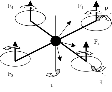
The considered system is shown in figure 1 where rotors one and three are clockwise while rotors two and four are counter clockwise. In appendix the dynamics of the rotors are briefly characterized.

The main simplifying assumptions adopted with respect to flight dynamics in this study are a rigid cross structure, no wind, negligible aerodynamic contributions resulting from translational speed, no ground effect as well as negligible air density effects and very small rotor response times. It is then possible to write simplified rotorcraft flight equations [6]. The moment equations can be written as:

) (

) / (

) ( ) / (

) ( ) / (

3 4 1 2

4 3 1

2 2 4

F F F F I k r

r p k F F I a q

r q k F F I a p

zz yy xx

− + − =

+ − =

+ − =

& & &

(1)

[image:1.595.322.509.448.602.2]

where p, q, r are the components of the body angular

Fig 1. Four rotor aircraft

speed, with k2(I_zz−I_yy)/I_xx and k4=(Ixx−Izz)/Iyy, Ixx, Iyy

and Izz being the moments of inertia in body-axis and m the

total mass of the rotorcraft. The Euler equations are given by:

r q

r q

r q

p

)) cos( / ) (cos( ))

cos( / ) ((sin(

) sin( ) cos(

) cos( ) tan( ) sin( ) tan(

θ φ θ

φ ψ

φ φ

θ

φ θ φ

θ φ

+ =

− =

+ +

=

& & &

(2)

where θ, φ, and ψ are respectively the pitch, bank and heading angles.

I

F4 F1 _p

F2

F3

The acceleration equations written directly in the local Earth reference system are such as:

F M g z F m y F m x ) cos( ) cos( ) / 1 ( )) sin( ) cos( ) cos( ) sin( ) )(sin( / 1 ( )) sin( ) sin( ) cos( ) sin( ) )(cos( / 1 ( φ θ φ ψ φ θ ψ φ ψ φ θ ψ + − = − = + = && && && (3)

where x, y and z are the centre of gravity coordinates and where :

4 3 2

1 F F F

F

F= + + + (4) and with the constraints:

{

1,2,3,4 0≤F ≤Fmax i∈

i

i

}

(5) III. NLICONTROL APPROACH FOR TRAJECTORY TRACKING

Here we are interested in controlling the four rotor aircraft so that its centre of gravity follows a given path with a given heading ψ while attitude angles θ and φ remain small. Many potential applications require not only the centre of gravity of the device to follow a given trajectory but also the rotorcraft to present a given orientation.

A. Attitude Control

From equations (1) it appears that the effectiveness of the rotor actuators is much larger with respect to the roll and pitch axis than with respect to the yaw axis. Then it is considered here that attitude control is involved with controlling the θ and φ angles. In equations (1) the effect of rotor forces appears as differences so, we define new attitude inputs u1 and u2 as:

3 1

1 F F

u = −

u

₂

=

F

₂

−

F

₄ (6.1) In the heading and position dynamics, the effects of rotor forces and moments appear as sums, so we define new guidance inputs v1and v2 as:

3 1

1

F

F

v

=

+

v

₂

=

F

₂

+

F

₄ (6.2) It is supposed that u1 and u2 can be made to vary

significantly while v1 and v2 can remain constant.

Then the attitude dynamics can be rewritten under the affine input form: U X g V X f

X&= ( , )+ ( ) (7.1) Y'=(θ,φ) (7.2) with ) , , , (

' p qθ φ

X = , U'=(u1,u2) andV'=(v1,v2) (8)

Then, taking profit of non linear inverse control theory, it appears that all the attitude angles have relative degrees equal to one and that there is no internal dynamics while the output equations can be rewritten as:

) ( ) ( )

(Y U N X V P X

M

Y&&= + + (9)

with ⎥ ⎦ ⎤ ⎢ ⎣ ⎡ − = xx yy yy I a I tg a I a Y M / / sin 0 / cos )

( _θ φ_φ (10)

⎥ ⎦ ⎤ ⎢ ⎣ ⎡ − − = zz zz zz I tg k I tg k I k I k X N / cos / cos / sin / sin ) ( φ θ φ θ φ

φ ₍₁₁₎

]' , [ ) (X P₁ P₂

P = where: )) cos sin ( ( ) cos sin ( cos 4 1 φ θ φ θ φ φ φ tg r q tg p r q r p k P + + + − = (12.1) dt tg d r dt tg d q tg r p k r q k P / ) cos ( / ) sin ( sin 4 2 2 φ θ φ θ φ θ + + + = (2.2)

Then, while φ≠±π/2, the attitude dynamics given by (9) are invertible. Then it appears opportune to adopt as a partial control objective to assign to the attitude angles second order linear dynamics towards their current reference values: ⎥ ⎥ ⎦ ⎤ ⎢ ⎢ ⎣ ⎡ − − − − − − = = ⎥ ⎦ ⎤ ⎢ ⎣ ⎡ ) ( 2 ) ( 2 2 2 c c d d d _Y φ φ ω φ ω ζ θ θ ω θ ω ζ φ θ φ φ φ θ θ θ & & && &&

&& ₍₁₃₎

where

ζ

_θ,

ζ

_φ,

ω

_θ,

ω

_φ are respectively damping and natural frequency parameters while θc and φc are reference

values for the attitude angles. Then the resulting non linear inverse attitude control law is given by:

) ) ( ) ( ( )

(Y 1 N X V P X Yd

M

U=− − + − && (14) B. Guidance Control Law

Considering that the attitude dynamics are stable and much faster than the guidance dynamics, the guidance equations can be approximated by the control affine form:

⎥ ⎥ ⎥ ⎥ ⎥ ⎥ ⎦ ⎤ ⎢ ⎢ ⎢ ⎢ ⎢ ⎢ ⎣ ⎡ + + − + − + + − = ⎥ ⎥ ⎥ ⎥ ⎥ ⎦ ⎤ ⎢ ⎢ ⎢ ⎢ ⎢ ⎣ ⎡ ) ( ) cos( ) cos( ) / 1 ( ) ( )) sin( ) cos( ) cos( ) sin( ) )(sin( / 1 ( ) ( )) sin( ) sin( ) cos( ) sin( ) )(cos( / 1 ( ) ( cos cos 2 1 2 1 2 1 1 2 v v m g v v m v v m v v I k z y x c c c c c c c c c zz c φ θ φ ψ φ θ ψ φ ψ φ θ ψ θ φ ψ && && && && (15)

Here also, the outputs of the guidance dynamics present relative degrees equal to 1 while the internal dynamics, which are concerned with the attitude angles are supposed already stabilized. Then, considering that second order linear dynamics are also of interest for the guidance variables, we can define desired accelerations by:

⎥ ⎥ ⎥ ⎥ ⎥ ⎦ ⎤ ⎢ ⎢ ⎢ ⎢ ⎢ ⎣ ⎡ − − − − − − − − − − − − = ⎥ ⎥ ⎥ ⎥ ⎦ ⎤ ⎢ ⎢ ⎢ ⎢ ⎣ ⎡ ) ( 2 ) ( 2 ) ( 2 ) ( 2 2 2 2 2 c z z z c y y y c x x x c c c c c z z z y y y x x x z y x ω ω ζ ω ω ζ ω ω ζ ψ ψ ω ψ ω ζ

ψ _{ψ ψ ψ}

& & & & && && && && (16)

where ζψ,ζ_x,ζ_y,ζ_z,ωψ,ω_x,ω_y,ω_zare respectively damping

and natural frequency parameters while ψc, xc, yc and zc are

reference values for the attitude angles. Of course, many other schemes can be proposed to define desired accelerations at the guidance level.

) cos

cos )

( (

2

1 2 2 2

1 c

c c zz c

c c

k I g z y x m

v ψ

φ θ

&& &&

&&

&& + + + −

= (17.1)

) cos

cos )

( (

2

1 2 2 2

2 c

c c zz c

c c

k I g z y x m

v ψ

φ θ

&& &&

&&

&& + + + +

= (17.2)

with

)) /( ) sin cos

((x y z g

arctg _{c c c}

c= && ψ+ && ψ && +

θ (18.1)

and

2 2

2

) (

cos sin

arcsin(

g z y x

y x

d d d

d c

c

+ + +

− =

&& && &&

&& && ψ ψ

φ (18.2)

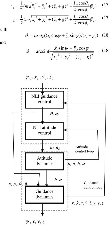
p, q, θ, φ

[image:3.595.49.283.50.533.2]

ψ

,

x

,

y

,

z

Fig 2. Proposed control structure

Then, returning to the expression of the attitude control law , it happens that the centre of gravity acceleration terms compensate each others and the law becomes simply:

) ) ( ) ( ( )

( 1

d

Y X P X N Y M

U =− − + − && (19) with

c

c c

c c

N N X

N ψ

φ φ θ θ θ

φ φ θ

&& ⎥ ⎥ ⎥ ⎥

⎦ ⎤

⎢ ⎢ ⎢ ⎢

⎣ ⎡ − = ⎥ ⎦ ⎤ ⎢ ⎣ ⎡ =

cos cos cos cos sin

cos sin cos )

(

2 1

(20)

The whole proposed control structure is given in the above figure 2.

IV. FLIGHT CONTROL SUPERVISION

Since the above control approach does not consider explicitly the input level constraints, we introduce here a supervision layer whose function is to avoid the generation

of unfeasible reference values for the inputs by modifying, as less as possible, the current control objectives. According to (5), (6) and (7), the control signals should be such as:

2 , 1

max

max≤ ≤ =

−F ui F i (21.1) and 0≤vi≤2Fmax i=1,2 (21.2)

Conditions (21.1) implies for the desired attitude accelerations to satisfy the following conditions:

max

min φ φ

φ&& _≤ &&_{c ≤} && _(22.1) with

max 2

2 min

cos

F I a P N

yy φ

φ&& = + − (22.2) and

max 2

2 max

cos F I a P N

yy φ

φ&& = + + (22.3) and condition:

max

min θ θφ θ

θ&& ≤ &&_c−tg &&_c ≤ && (23.1) with

) ( ) (

/ 1 1 2 2

max

min =−aF Ixx+ N +P −tgθ N +P

θ&& (23.2)

and

) ( ) (

/ 1 1 2 2

max

max=aF Ixx+ N +P −tgθ N +P

θ&& (23.3)

Then, reference values for instant attitude angles accelerations can be obtained from the solution of the following linear –quadratic optimization problem:

2

2 _{( )}

) (

min θ α φ β

β

αr c− + c−

&&

&& _(24.1) with

max

min

β

φ

φ

&& ≤ ≤ && (24.2)

max

min α θ β θ

θ&& ≤ −tg ≤ && (24.3)

Observe that the solution of this problem is equal to ( ) if it is feasible with respect to constraints (24.2) and (24.3), otherwise the solution will be on the border of the convex feasible set.

c cφ

θ&&_, &&

Then if α*and β*are solution of this problem, u1 and u2 are

given by:

) ) ( ) ( ( ) (

* * 1

2 1

⎥ ⎦ ⎤ ⎢ ⎣ ⎡ − + −

= ⎥ ⎦ ⎤ ⎢ ⎣

⎡ −

β α

X P V X N Y M u u

(25) In the case of v1 and v2 (relations (21.2)) and considering the

expressions of θc and φc the above approach leads to the

consideration of an intricate non convex optimization problem. A different approach is proposed here. Let λ be such as:

) ( ,

,y y z g z g

x

x&&r =λ &&c &&r =λ &&c &&r+ =λ &&c+ (26)

then according to (18.1) and (18.2):

c

r θ

θ = and φ_r =φ_c (27) Feasible reference values for

x

&&

_r,

y

&&

_r,

z

&&

_r and

ψ

&&

_rcan be obtained from the solution of the following linear –quadratic optimization problem:

2 2 2 (28.1)

, ( 1) ( )

min λ η μ ψ_c

μ

λ − + − &&

with Attitude

dynamics

Guidance dynamics NLI attitude

control NLI guidance

control

z y x z y x

r,ψ&,&,&,&, , , θc,φc

c c c c x&& y&& z&&

&& , , ,

ψ

u1,u2

v1 ,v2, θc, φc

θ, φ

Attitude control loop

max 2

2 2

4 ) cos

cos ( ) ) ( (

0 F

k I g z y x m

c c zz c

c

c + + + − ≤

≤ μ

φ θ λ

&& &&

&& (28.2)

max 2

2 2

4 ) cos

cos ( ) ) ( (

0 F

k I g z y x m

c c zz c

c

c + + + + ≤

≤ μ

φ θ λ

&& &&

&& (28.3)

where η is here a time constant. Let and be the solution of the above problem, then the control inputs can be taken as:

*

λ μ*

) cos

cos )

( (

2

1 * 2 2 2 *

1 _φ μ

θ λ

c c zz c

c c

k I g z y x m

v = && + && + && + − (29.1)

) cos

cos )

( (

2

1 * 2 2 2 *

2 _φ μ

θ λ

c c zz c

c c

k I g z y x m

v = && + && + && + + (29.2) Then, F₁,F₂,F₃,F₄ given by:

2 / ) ( 1 1 1 u v

F = + F2 =(u2 +v2)/2 (30.1) 2

/ ) ( _{1 1} 3 v u

F = − F4 =(v2 −u2)/2 (30.1) satisfy condition (5).

V. CASE STUDIES

Here we considered two cases: one where the objective is to hover at an initial position of coordinates x0, y0, z0

while acquiring a new orientation ψ1, and one where the

rotorcraft is tracking the helicoïdal trajectory of equations: t

t

xc()=ρcosν t

t

yc()=ρsinν

t

z_c =δ+γ (31) 2

/ )

( ν π

ψc t = t+

where ρ is a constant radius and γ is a constant path angle.

A. Heading control at hover

In this case we get the guidance control laws: )

( 2 1

1 zz c

k I g m

v = − ψ&& ( ) 2

1

2 zz c

k I g m

v = + ψ&& (32) with the following reference values for the attitude angles:

0

= c

θ and φ_c=0 (33) Here the heading acceleration is given by:

) (

2 1

2_{ψ ψ}

ω ω ζ

ψ&&c =− _{ψ ψ}r− _ψ − (34)

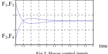
Starting from an horizontal attitude ( θ(0)=0, φ(0)=0), attitude inputs u1 and u2 given by relation (14) remain equal

to zero. Then, figures 3 and 4 display some simulation results:

0 0 . 5 1 1 . 5 2 2 . 5 3 3 . 5 4 4 . 5 5

[image:4.595.38.533.46.537.2]

0 5 1 0 1 5

Fig 3. Hover control inputs

0 0 . 5 1 1 . 5 2 2 . 5 3 3 . 5 4 4 . 5 5

0 0 . 2 0 . 4 0 . 6 0 . 8 1 1 . 2 1 . 4 1 . 6 ψ-ψc

time

Fig 4. Heading response during hover

B. Trajectory tracking case

In this case we get the guidance control laws:

) (

2

1 2 2 2

2

1 v m g

v = = ρν + (38)

Here the permanent reference values for the attitude angles are such as:

0 =

c

θ (39.1) and

2 4 2

2 sin

g c

+ − =

ν ρ

ν ρ

φ (39.2) and the desired guidance and orientation accelerations are given by:

0 , 0

) sin(

) cos( 2 2

= =

− =

− =

c c

c c

z

t y

t x

ψ ν ν ρ

ν ν ρ

&& &&

&& &&

(40)

Attitude inputs are given by relation (14) where now:

⎥ ⎦ ⎤ ⎢

⎣ ⎡

− =

−

a I a I tg tg

a I M

xx xx

yy

/ /

0 ) cos /( 1

φ θ

φ ₍₄₁₎

and

[

0 0 )'

(X =

N

]

(41) In figures 5 to 7 simulation results are displayed where at initial time the rotorcraft is hovering:

y(t

-2 . 5 -2 -1 . 5 -1 -0 . 5 0 0 . 5 1 1 . 5 2 2 . 5 -2 . 5

-2 -1 . 5 -1 -0 . 5 0 0 . 5 1 1 . 5 2 2 . 5

[image:4.595.348.509.558.640.2]

x(t) Fig 4. Evolution of rotorcraft horizontal track

F1,F3

0 0 . 5 1 1 . 5 2 2 . 5 3 3 . 5 4 4 . 5 5 0

0 . 0 2 0 . 0 4 0 . 0 6 0 . 0 8 0 . 1 0 . 1 2 0 . 1 4

z(t

F2,F4

time

[image:4.595.65.245.686.777.2]

0 0 .5 1 1. 5 2 2 .5 3 3. 5 4 4 .5 5 0

[image:5.595.344.490.50.208.2]

2 4 6 8 1 0 1 2 1 4

Fig 7. Rotorcraft trajectory tracking inputs

VI. CONCLUSION

In this communication a nonlinear inverse control technique applied to rotorcraft trajectory tracking has been considered. This approach leads to the design of a two level control structure based on analytical laws. However the possibility of actuators saturation has led to the design of a supervision layer whose objective is to modify references values for the nonlinear inverse control laws so that the tracking performance is maintained as much as possible. The applicability of the proposed approach appear acceptable since the complexity of the resulting optimization problems to be solved online appear to be rather low. Then the proposed approach should enlarge the field of applications for rotorcraft. This approach could be adapted to the supervision of actuators saturation with other autonomous aircraft.

APPENDIX

The rotor engine dynamics are characterized by the relation between the input voltage Va and the angular rate ω. A

possible model of rotor dynamics is given by:

) ( ) / ( ) ( ) ( 1 )

(t τωt KQωt 2 KVa τ Va t

ω& =− − + (A.1)

with ω(0)=ω₀ , where τ , KQ and KVaare given positive

parameters and where the voltage input is such as: max

0≤Va ≤V (A.2) with a negligible time response for the voltage generator. The step response (Va =constant) of the rotor is solution of

the scalar Riccati equation:

a V

Q t K V

K t

t) 1 () () ( _a/ )

( ω ω 2 τ

τ

ω& =− − + (A.3)

with ω(0)=ω₀ .

A particular solution ω1 of the associated differential

equation is such as:

( 1 4 1)

2 1

1= + V Q a −

Q

V K K

K a τ

τ

ω (A.4) In the general case, the solution of (A.3) can be written as

' / ' / 1

1

) 1 ( ' )

0 (

1 1 )

( τ

τ

τ ω ω ω

ω t

t Q

e e K

t −

−

− +

− +

= (A.5)

(A.6)

and (A.7) 1

) ( limω =ω

+∞ → t

t

F2,F4

0 .1 .2 .3 .4 .5 .6 .7 .8 .9 1

1.5 2 2.5

Omega (rad/s) Va=2

0 .1 .2 .3 .4 .5 .6 .7 .8 .9 . 1

0 5 10 15

omega (rad/s) Va=20

F1

F3 time

Fig 8. Two examples of rotor step response

It appears from figure 8 that the dynamics of the rotor may be close to those of a first order linear system with time constant τ’, but as can be seen in (A.6), this value is a function of Va. If the desired dynamics for the output are

such as:

1_{( )}

c

T ω ω

ω&=− − (A.8) where T is a very small time constant Va can be chosen such

as: )

) ( )

( ) 1 (( 1 )

( _{K t} 2

T t T K t

V _{c Q}

V a

a

ω τ ω τ ω τ

+ + −

= (A.9)

The rotor forces are then given by:

4 1

2

to i f

F_i =

ω

_i = (A.10) while the rotor moments are given by:

4 1to i F k

Mi = i = (A.11)

where f and k are positive constant parameters.

REFERENCES

[1] G. Hoffmann, D.G. Rajnarayan, S.L. Waslander, D. Dostal , J.S. Jang, and C.J. Tomlin, “The Standford Tetsbed of Autonomous Rotorcraft

for Multi-Agent Control”, 23rd _{Digital Avionics Systems Conference,}

Salt Lake City, UT, November 2004.

[2] H. K. Khalil, “Nonlinear Systems”, Prentice Hall, 3rd Ed., 2002. [3] S.N. Singh and A.A. Schy, “Nonlinear decoupled control synthesis for

maneuvring aircraft”, Proceedings of the 1978 IEEE conference on Decision and Control, Piscataway, NJ, 1978.

[4] R. Ghosh and C.J. Tomlin., “Nonlinear Inverse Dynamic Control for

Model-based Flight”, Proceeding of AIAA-GNC, 2000.

[5] R. Asep, T.J. Shen, and F. Mora-Camino, “An application of the

nonlinear inverse technique to flight-path supervision and control”,

Proceedings of the 9th International Conference of Systems Engineering, Las Vegas,NV, 1993.

[6] B. Etkin, and L. R. Reid, “Dynamics of Flight-Stability and Control”.

John Wiley & Sons. New York, NY, 1996.

[7] W.C. Lu, and F. Mora-Camino, “Flight Mechanics and Differential Flatness”. Dincon 04, Proceedings of Dynamics and Control Conference, Ilha Solteira, Brazil, pp. 830-839, 2004.

[8] A.Drouin, A.B. Ramos and F. Mora-Camino, “Rotorcraft Trajectory Tracking by Nonlinear Inverse Control”, Dincon, São Paulo, 2007. [9] S.A. Beltran Mendoza, O. Lengerke,H. Gonzalez Acuña and F.

Mora-Camino, “Control PID de altura de un quadrirotor” , 3rd International Mechatronic Conference, Bucaramanga, Colombia, October 2011.

a Q

VK V

K τ

[image:5.595.65.248.76.174.2]