Increasing the Performance of a Training Algorithm for Local Model Networks

Increasing the Performance of a Training

Algorithm for Local Model Networks

Torsten Fischer, Benjamin Hartmann and Oliver Nelles

Abstract—In this paper the improvement of the established training algorithmHILOMOT is presented.HILOMOT is a hierar-chical tree-construction method based on the ideas of neuronal networks and fuzzy-systems and an advancement of the well-knownLOLIMOT-Algorithm. During the training the input space is divided into subregions with the help of validity functions. This is done iteratively by splitting the current worst local model, until an specified exit condition is reached. For every subregion one local linear model is estimated by a weighted least squares method. The main purpose is keeping the number of local models low. Therefore the split position is optimized during the training. The optimization problem is nonlinear, so a gradient-based nonlinear local optimization method, called Quasi-Newton method, is used. The main drawback of this approach is its long calculation time. The most time consuming part is the numerical calculation of the gradient done by the finite difference technique.To avoid this problem the numerical approach is replaced by the analytical gradient. This leads to a significant reduction of the training time without decreasing the approximation quality.

Index Terms—neuronal networks, fuzzy-logic, system identi-fication, nonlinear optimization.

I. INTRODUCTION

M

OST of the commonly used methods in automatic control engineering require a well formulated model of the system in order to be controlled. Many real pro-cesses are too complex to use an analytical model. In these cases the experimental modeling, called identification

is employed. Commonly used identification methods are neuronal networks and neuro-fuzzy systems. A method based on this ideas is the HILOMOT(HIerachical LOcal MOdel

Tree)-Algorithm [6], which can be seen as an advance-ment of the well-known LOLIMOT(LOcal LInear MOdel

Tree)-Algorithm [5], [7]. In Contrast to LOLIMOT, which uses orthogonal Gaussian membership functions for the partition, HILOMOT uses arbitrarily orientated Sigmoids. Consequently they are more flexible during the training and a better indication of the nonlinear characteristics of the process is afforded [3]. The price of a lager flexibility is a required nonlinear optimization, which is necessary in order to get the best segmentation of the input space with respect to the training error. One way to improve the performance of HILOMOT significantly in terms of training time is the application of an analytical gradient instead of a numerically derived gradient information. This paper increases the performance of the algorithm by improving this optimization procedure. Therefore, first a brief overview of the mode of operation of the HILOMOT Algorithm is given. Then the optimization of the split function used for

T. Fischer, B. Hartmann and O. Nelles are with the Depart-ment of Mechanical Engineering, University of Siegen, Germany, email: [email protected], [email protected], [email protected]

partitioning is discussed and the difficulties are identified. The implemented approaches to overcome this problems are illustrated and the modifications are compared and evaluated to the optimization method used in an empirical examination so far. Different example processes are investigated.

II. PRINCIPLEOPERATION OF THEALGORITHM

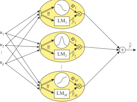
[image:1.595.311.544.500.674.2]

The basic idea of HILOMOT is the description of the training data with local sub-models of polynomial type. These local models are interpolated with so called validity functions. The local models are linearly parameterized, i.e. can be estimated with weighted least squares. In contrast to the local models, the validity functions contain nonlinear parameters. Therefore, these parameters only can be found by iterative methods. Other algorithm like CART [2] or LOLIMOT[5], [7] are popular methods that also follow this strategy too. These algorithms are heuristic tree-construction methods. They use heuristical approaches for finding the structure parameters in contrast to the HILOMOT, which performs a nonlinear optimization of its structure param-eters. Therefore, they are much faster, but have a lower flexibility concerning the split position and direction. The general principle of all of them (Fig. 1) can be interpreted as a fuzzy model in Takagi-Sugeno form, which are very important for approximation strategies for nonlinear static and dynamic processes [1], [4]. The global model output yˆ

Fig. 1. Local model network: The outputyˆiof each local model is weighted

by its validity functionΦiand summed up to the global model outputy.ˆ

is a superposition of weighted local models, where each of theM local models is a rule in terms of fuzzy logic:

ˆ

y= M X k=1

ˆ

Here, the local modelsyˆkare the associated rule consequents and the validity functions Φk represent the rule premises, with the vector z spanning the premise input space and the vector x spanning the consequent input space. They result from the input vector uof the real process, as illustrated in Fig. 2. By dealing with independent input spaces for the rule

...

u1

u2

up

general model

premises

consequents z1

z2

znz

...

x1

x2

xnx

...

y

y Fi

Fig. 2. The input vectoruof the general nonlinear model, can be assigned to the premise (nonlinear) and/or consequent (linear) input space according to their influence of the output behavior.

premises and consequents, it is possible to incorporate prior knowledge about the nonlinear behavior between each input and the output into the model structure. Each local modelyˆk is defined by its parameter vectorw_k and the vector x:

ˆ

yk=x·wk. (2)

The parameters of the local models can be easily estimated by an local or global least-squares method, if the validity functionsΦk are known. The local estimation of the param-eter vectorw_k is:

w_k =XT·Q

k·X −1

·XT ·Q

k·y . (3) Here matrix Q

k is a diagonal matrix including the weights of the k-th local model, which are its validity function Φk, and matrix X is the input matrix of the consequent input space, whose columns represent one data point.

As mentioned in the introduction, HILOMOTuses sigmoids as splitting functions in contrast to LOLIMOT, which applies orthogonal gaussians. The arbitrary orientation of the sig-moids in the premise input space is their advantage [3]. A sigmoid is described by:

Ψ(z) = 1

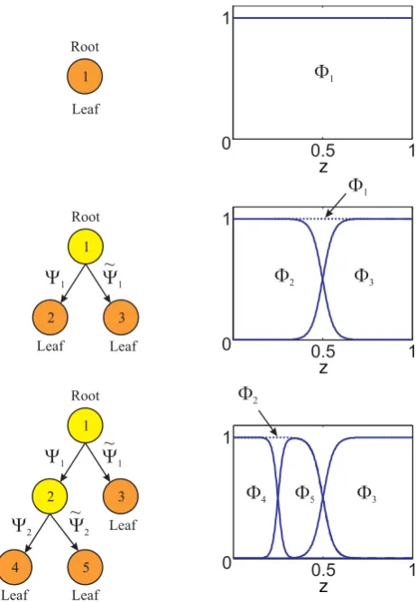
1 +e(v0+z1·v1+...+znz·vnz) , (4) where vector v contains the parameters of the sigmoid and the vector z spans the premise input space, whose number of inputs isnz [5], [6]. A typical partitioning done over the first training iterations of HILOMOT is shown in Fig. 3. A split is realized by dividing the validity area of the worst local model into two sub-models by a sigmoid Ψ1 and

its complementary function Ψ˜1. Each validity function is

a product of all sigmoid function along the path beginning at the root and ending in the leafs. The complexity of the global model increases in each iteration, which means that a better approximation is achieved step by step. In order to get a good approximation with as less local models as possible, in each iteration the parameters of the new sigmoid are optimized. To guarantee a good initialization for the nonlinear optimization, all orthogonal splits are done in the premises input space and the best one with respect to the used global loss function is chosen as starting point. To

z

[image:2.595.312.543.50.384.2]

z z

Fig. 3. Tapical tree structure: Splitting the worst local model in each iteration. The validity function of each leaf results from the multiplication of the all sigmoids functions along the path.

[image:2.595.53.289.139.232.2]

assess the optimization problem precisely, a closer look on the properties of a sigmoid has to be taken. The parameters of the sigmoid influence its position and steepness. The position of the sigmoid corresponds to the position of the split, which is taken during the training. The steepness spec-ifies the smoothness of the transition between the adjoining local models. In order to discuss these statements in detail, Fig. 4 shows a schematic illustration of a two-dimensional Sigmoid. The level curve atΨ(u1, u2) = 0.5 of the sigmoid

0 0.2 0.4 0.6 0.8 1

0 0.2 0.4 0.6 0.8

1

z₂

v₁

v₂

v₀ v1 v0

v₂

v₀

v12+v22

cutting edge

1 x 2

x

v*

1

[image:2.595.317.538.577.758.2]

z

describes the splitting line, where the change of the bigger validity between both local models is given. For a higher dimensional premise input space the partitioning is done by hyperplanes. The direction of the split is described by the vector v∗ = [v1, v2, . . . vnz], which is called direction vector. The difference between the parameter vector v and the direction vector v∗ is the parameter v0. The orthogonal distance of the hyperplane to the origin is described by the ratio v0/kv∗_{k. With the direction and the distance the}

position of the split is defined accurately. Another possible representation can be done by vectors along the axes of the premise input space. They define the intersection xj of the splitting line with the corresponding axis. Here we got two input dimensions and according to this the points x1

und x2, with x1 = v0/v1 and x2 = v0/v2. It is obvious

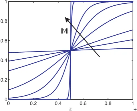
that the position of the sigmoid can be defined only by the ratios of the parameters. The length of the vector specifies the steepness of the sigmoid, and therewith the character of the continuous transition between the local models. This relationship is shown in Fig. 5. Here several one-dimensional

0 0.2 0.4 0.6 0.8 1

0 0.2 0.4 0.6 0.8 1

z v

[image:3.595.49.289.305.500.2]

+

Fig. 5. One-dimensional sigmoids with different transitions.

sigmoids are illustrated, that all have the same point of intersection. The parameter vectors of the sigmoids differ only in their length, whereupon the ratios between the single parameters stay the same. The length of the parameter vectors of the sigmoids increases along the direction of the arrow. In summary, the ratio between the single parameters indicates the position of the sigmoid, which is the same as the position of the split and the length of the parameter vector defines the steepness of the sigmoid, which describes the smoothness of the transition between the adjoined local models. In LOLIMOT, the choice of the parameters of the gaussian results from heuristic geometrical considerations, which are easy to perform [5]. HILOMOT however uses arbitrary orientated sigmoids, whose nonlinear parameters can not result from heuristically approaches. Thats why they need to be optimized to reach a minimal number of local models to describe the process. The optimization is performed by the Quasi-Newton-Method, which belongs to the group of nonlinear local gradient-based optimization methods [5], [9]. Optimizing the parameter vector v leads to a very steep slope and a very hard transition between the

local models. Using local estimation, this is the best solution in terms of the considered loss function. A hard transition is not intended. Therefore, the influence of the parameters on the steepness of the sigmoid needs to be removed by a standardization of the length of the vector v [6]. Hence, a parameter κ is introduced, which directly influences the sharpness of the transition:

κ= 20

p

v·vT _· q

∆c·∆cT·σ

= 20

kvk · k∆ck ·σ . (5)

Combined with Eq. (4) follows:

Ψ(z) = 1

1 +eκ·(v0+z1·v1+...+znz·vnz)

= 1

1 +eκ·(v0+z·v∗) . (6)

The distance of the centers of the adjoined local models ∆c and the smoothness parameter σ, which is used to calibrate the overall transition behavior, are responsible for the steepness of the sigmoids [6]. The influence of the parameter vector v on the steepness is abrogated by the division with the norm of the vector included inκ.

III. PROBLEMSTATEMENT ANDAPPROACHES

As mentioned before, the parameter κ neglects the in-fluence of the parameter vector v on the smoothness of the transition between the local models by normalizing it. Thus, only the position of the split remains affected by the vectorv. Needing just the ratios of the parameters to define the exact position, one parameter becomes redundant. If the optimizer considers the whole vector v, it handles a over-determined optimization problem. This proceeding causes a long calculation time and possibly a worse result. To avoid this, one parameter must be fixed during the optimization. Generally it is irrelevant which parameter is chosen. A good one is the offset v0, because it is clearly separated form

the premise input space matrix and the other parameters in Eq. (6). By fixing the parameter v0, the problem is not over-determined anymore and reduced by one dimension. Hence, the performance of the optimizer and of the whole algorithm increases. In order to optimize the parameters, the Quasi-Newton-Method is used, which needs the gradient of the loss function I. If an analytical gradient is not given, a numerical approach is needed. The numerical calculation of the gradient, which the Quasi-Newton-Method typically uses, is done by the finite difference technique. Its drawback among other issues is its high computational effort with respect to number of parameters to be optimized [5], [9]. In order to avoid this problem, an analytical gradient should be implemented. The loss function appropriated by HILOMOTis the NRMSE(NormalizedRoot MeanSquaredError):

I(θ) = s

N P i=1

e2

i(θ)

s N P i=1

(yi−y)

2

. (7)

This means the general equation of the gradient has to be changed into:

g(θ) =∂I(θ)

∂θ =g(v

∗_{) =}∂I(v∗)

∂v∗ . (8)

Here, the gradient consists of the derivatives with respect to each sigmoid parameter. Thus, thej-th entry of the gradient for thej-th sigmoid parameter can be specified by:

gj = N X i=1

(yi−y)

2

!−12

· ∂

∂vj N X i=1

e2_i(vj) !12

, (9)

where N is the number of data samples, yi is the output at the i-th data sample, y = _N1 P

yi the mean of all data samples and ei(vj) = yi−yˆi(vj) is the error at the i-th data sample. Because just the global model is addicted to the vectorv∗ Eq. 9 becomes:

gj =−F1·

N X

i=1 ei·

∂yˆi(vj)

∂vj

, (10)

In Eq. (10) a placeholder F1 is used for a more compact

formulation:

F1=

N X

i=1

(yi−yˆ)

2

!−12

· N X i=1

e2_i

!−12

. (11)

The estimation of the parameters of the local models is performed by a weighted least squares approach and these weights result from the validity areas of the local models [6]. Furthermore the normalization of the parameters is done, which leads to additional terms in the gradient equation. After considering this addictions the following expression for each entry of the gradient results:

gj=

∂I ∂vj

=

−F1· N X i=1

ei·Φ∗i ·

(ˆya,i(θ)−yˆb,i(θ))·

∂Ψi

∂vj

+X_i·XT ·Q

a·X −1

·XT ·∂Qa

∂vj ·

h

y−ˆy_ai·Ψi(θ)

−Xi·

XT ·Q_b·X

−1

·XT ·∂Qa

∂vj ·

h

y−ˆy

b i

·Ψ˜i(θ) o

. (12)

Φ∗

i is the validity function of the local model, which is split. ˆ

ya,i and yˆb,i are the new local models arising out of the currently worst local model by splitting. The split is done by the sigmoidΨi and its complementary functionΨ˜i:

˜

Ψi= 1−Ψi. (13)

Q_a and Q_b are the weighting matrices of the new local models. The calculation of the derivatives of the weighting matrix Q and of the sigmoids are done separately, because the equation would be too long and confusing. The deriva-tives of the weighting functions only vary in their sign:

∂Q_a

∂vj

=−∂Qb

∂vj

. (14)

Hence, it is just necessary to calculate the derivation of the diagonal weighting matrixQ

a as: ∂Q a ∂vj =     Φ∗ 1·

∂Ψ1

∂vj . . . 0 ..

. . .. ... 0 . . . Φ∗_N ·∂ΨN

∂vj     . (15)

In Eq. (12) and (15) the derivative of the sigmoid needs to be calculated. Eq. (16) shows the associated formula. Because of the normalization of the parameter vector inside the exponential function, the equation is not really well formulated. Hence, two more placeholders are added in order to achieve a shorter expression:

F2,i=

eκ(v0+Zi·v

∗₎

1 +eκ(v0+Zi·v∗)

2 , (17)

and

F3=−20

σ ·(kvk · k∆ck)

−2

. (18)

In Eq. 17 the matrix Z is the input matrix of the premise input space and its i-th column Z_i represent the i-th data point. With the equations above, the derivative of each parameter of the vectorv∗ is clearly defined. This incorpo-rates the derivative of the sigmoid and the derivative of the weighting matrix. Obviously the calculation of the analytical gradient depends on the number of data points. The formula is analytical, but it is evaluated at discrete points. Thereby its vulnerable to low number of data points or scattered data points, which at worst causes the optimizer to crash. To guarantee a robust modeling and therewith a deterministic approximation, the orthogonal initial split has to be used, if the nonlinear optimization fails.

IV. VALIDATION

To demonstrate the increased performance of the algorithm by the modification explained in the last section, three example processes are modeled and the results are compared against each other. The examples are a symmetric hyperbola and parabola, and the so called ”radcos”-function, which was used during a dissertation to verify its results [8]. The formula for two input dimensions of the ”radcos”-function is

y= cos

9·qu2

1+u22+ 2

+

1

2 ·cos (11·u1+ 2) + (19) 15·(u1−0.4)2+ (u2−0.4)2

2 ,

∂Ψi

∂vj

=−F2,i·     

κ·Zi,j+ (v0+Zi·v∗)·

vj· k_k∆_vc_kk−2· kvk

k∆ck·

n P l=1

∆cl·_N1 · N P k=1

ul,k·Φ∗k·F2,k·κ·Zk,j

1

F3 + 2· kvk k∆ck·

n P l=1

∆cl·_N1 · N P k=1

ul,k·Φ∗k·F2,k·(v0+Zk·v∗)     

. (16)

0

0.5

1

0 0.5

1 -2 0 2 4 6 8

u

1

u

[image:5.595.321.519.455.631.2]

2

Fig. 6. The ”radcos”–function with two input dimensionsu1andu2.

ten. Either the algorithms reach the error limit within the permitted number of local models or the maximum number of local models is used to gain the smallest possible NRMSE. The error values in Table I result from the given training data set. The quality of approximation is only slightly different

TABLE I

GLOBALERROR(NRMSE)OF THETRAININGDATASET INPERCENT. THEBESTVALUE INEACHCOMPARISON ISHIGHLIGHTED.

error [%] process num. grad anal. grad

2D hyperbola <5 <5

3D <5 <5

4D <5 <5

5D <5 <5

6D <5 <5

7D <5 <5

2D parabola 15.15 15.34

3D 24.84 24.77

4D 45.30 46.35

5D 59.93 59.80

6D 65.53 65.60

7D 70.42 70.62

2D radcos 18.05 17.30

3D 27.53 28.43

4D 37.9 38.33

5D 42.57 42.52

6D 44.76 44.93

7D 42.83 43.18

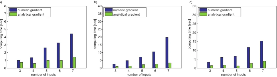
between both methods. It depends on the example, which method delivers the best result. Regarding a separate data set, which is used for validation, similar results can be observed, as Table II shows. Likewise the training data, no arbitrative differences in the quality of the approximation can be seen. The effect of the usage of the analytical gradient on both error values can be neglected. Regarding the computing time shown in Fig. 7 and Table III, dramatical changes arise.

For all three examples for every dimension of the input

TABLE II

GLOBALERROR(NRMSE)OF THETESTDATASET INPERCENT. THEBESTVALUE INEACHCOMPARISON ISHIGHLIGHTED.

error [%] process num. grad anal. grad

2D hyperbola 5.38 5.41

3D 4.93 4.82

4D 9.61 9.60

5D 4.43 4.54

6D 4.89 4.92

7D 3.15 3.18

2D parabola 14.94 15.12

3D 24.91 24.83

4D 46.55 46.59

5D 61.02 61.00

6D 68.49 68.51

7D 74.01 73.35

2D radcos 11.08 12.85

3D 28.90 29.69

4D 38.97 39.11

5D 44.12 43.80

6D 46.71 47.15

7D 46.90 46.65

space the analytical gradient has the lowest computational ef-fort. If the new implemented analytical gradient is used, the

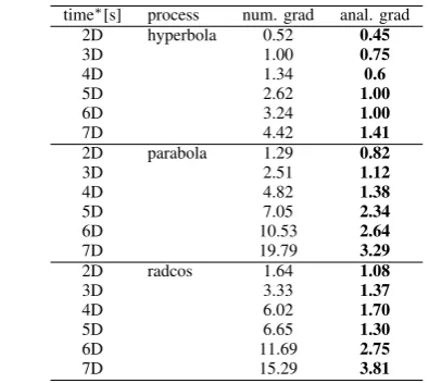
TABLE III

COMPUTIONTIME∗INSECONDS. THEBESTVALUE INEACH

COMPARISON ISHIGHLIGHTED.

.

time∗[s] process num. grad anal. grad

2D hyperbola 0.52 0.45

3D 1.00 0.75

4D 1.34 0.6

5D 2.62 1.00

6D 3.24 1.00

7D 4.42 1.41

2D parabola 1.29 0.82

3D 2.51 1.12

4D 4.82 1.38

5D 7.05 2.34

6D 10.53 2.64

7D 19.79 3.29

2D radcos 1.64 1.08

3D 3.33 1.37

4D 6.02 1.70

5D 6.65 1.30

6D 11.69 2.75

7D 15.29 3.81

∗_{Windows 7 (64-Bit), Intel Core i7 M 620 @ 2,67 GHz, 4,00 GB RAM}

computing time drops to 87% to 17% of the computing time with the numerical approach. Hence, the taken arrangements improve the performance of the algorithm considerably.

V. CONCLUSIONS

3 4 5 6 7 0

1 2 3 4 5 6 7 8

number of inputs

co

m

p

u

ti

n

g

ti

m

e

[se

c]

numeric gradient analytical gradient a)

3 4 5 6 7 0

5 10 15 20 25 30 35

number of inputs

co

m

p

u

ti

n

g

ti

m

e

[se

c]

numeric gradient analytical gradient c)

3 4 5 6 7 0

5 10 15 20 25 30 35 40

number of inputs

co

m

p

u

ti

n

g

ti

m

e

[se

c]

[image:6.595.61.537.52.185.2]

numeric gradient analytical gradient b)

Fig. 7. Computing times of the three methods with3to7input dimensions fora)the hyperbola, forb)the parabola and forc)the ”radcos”-function. The calculation was done by a computer using Windows 7 (64-Bit), Intel Core i7 M 620 @ 2,67 GHz with 4,00 GB-RAM.

HILOMOT, the NRMSE, with respect to the parameter of the sigmoid is done. The next modification is the imple-mentation of an analytical gradient of the loss function. The analytical calculated gradient makes the finite difference technique superfluous, which requires especially for high-dimensional input spaces a high computational effort [5]. The empirical examination shows, that the new implemented algorithm fulfills the expectations regarding the increase of performance . The computing time is reduced significantly and the quality of the approximation remains constant.

REFERENCES

[1] R. Babuˇska and H.B. Verbruggen. An overview of fuzzy modeling for control.Control Engineering Practice, 4(11):1593–1606, 1996. [2] L. Breiman and C.J. Stone J.H. Friedman R. Olshen R. Classification

and Regression Trees. Chapman & Hall, New York, 1984.

[3] B. Hartmann and O. Nelles. Advantages of hierarchical versus flat model structures for high–dimensional mappings. InWorkshop Com-putational Intelligence, Bommerholz, Germany, December 2009. [4] T.A. Johansen, R. Shorten, and R. Murray-Smith. On the interpretation

and identification of dynamic takagi-sugeno fuzzy models. Fuzzy Systems, IEEE Transactions on, 8(3):297–313, 2000.

[5] O. Nelles. Nonlinear System Identification. Springer, Berlin, Germany, 2001.

[6] O. Nelles. Axes-oblique partitioning strategies for local model net-works. In International Symposium on Intelligent Control (ISIC), Munich, Germany, October 2006.

[7] O. Nelles, S. Sinsel, and R. Isermann. Local basis function networks for identification of a turbocharger. In IEE UKACC International Conference on Control, pages 7–12, Exeter, UK, Sept. 1996. [8] J. Poland and A. Zell. Different criteria for active learning in neural

networks: A comparative study. In 10. European Symposium on Artificial Neural Networks, pages 119–124, 2002.