Online Full Text



Abstract— This paper presents a comparison between three

types of control algorithms for a 1.5 MW horizontal axis fixed speed wind turbine. It presents a fuzzy logic proportional integral control (Fuzzy PI), a fuzzy logic control (FLC) and a classical proportional integral (PI) control. Design of the proposed Fuzzy PI control algorithm was achieved via tuning with the Ziegler-Nichols approach at low and nominal wind speeds, using the same methodology for the PI controller tuning with the difference of incorporating a fuzzy logic section. The fuzzy logic section selects the desired PI gains according to wind speed with a smooth control transition. Fuzzy logic control was designed to obtain maximum power extraction at low wind speeds and to limit power extraction at 1.5 MW nominal power set point. Aerodynamic characteristics of the wind turbine were studied in order to gain a basic understanding of the system dynamics. A 1.5 MW horizontal axis wind turbine model with a squirrel cage induction generator model was designed for tuning as well as simulation performance studies. Simulation of the wind turbine was performed for two wind profiles, low wind speed and near nominal with fast wind speeds to test the controller’s response. Results demonstrate the effectiveness all techniques; appropriate responses were obtained for both simulation scenarios, achieving a controlled power extraction near the nominal value for the three controllers and maximum power extraction in low wind speeds for the Fuzzy PI and FLC control algorithms. A robustness test was performed by adding a normally distributed noise effect to wind speed input to the controllers, achieving good results for the Fuzzy PI control algorithm.

Index Terms—Wind power, fuzzy logic control, fuzzy

proportional integral control, proportional integral control.

I. INTRODUCTION

ONTROL algorithm design for renewable energy production is a topic of great concern nowadays

Manuscript received July 23, 2012; revised August 9, 2012. This work was supported in part by the Consejo Nacional de Ciencia Tecnología, CONACyT.

L. A. Torres Salomao is interin professor at Universidad Michoacana de San Nicolás de Hidalgo, Morelia, México. He is student at Centro de Ingeniería y Desarrollo Industrial, Santiago de Querétaro, México. (corresponding author, phone: +52 443 274 6570; e-mail: latsalomao@ieee .org).

H. Gámez Cuatzin is with Centro de Ingeniería y Desarrollo Industrial, Santiago de Querétaro, México (e-mail: [email protected]).

J. Anzurez Marín is with the Electrical Engineering Department, Universidad Michoacana de San Nicolás de Hidalgo, Morelia, México (e-mail: [email protected]).

I. I. Lázaro Castillo is with the Electrical Engineering Department, Universidad Michoacana de San Nicolás de Hidalgo, Morelia, México (e-mail: [email protected]).

because of all the efforts around the mitigation of greenhouse effects. Many countries have modified their energy production plans for the near future by advancing green energy technologies via government funding and tax reductions [1]. Wind energy is the technology with the most rapid growth, but since wind is an intermittent resource, efficiency of this machine is of outmost importance.

In Mexico, almost all installed wind turbines are of foreign design and construction, being fixed speed horizontal axis wind turbines the most common. Mexico presents zones like in La Ventosa, Oaxaca with wind persistence and speeds that make them some of the best installation sites in the world.

In practice, the majority of the installed wind turbines have pitch control systems with traditional Proportional – Integral (PI) algorithms. These control systems are designed near the nominal wind speeds and power extraction values because of their good response for linear model systems as well as their implementation simplicity. However, the dynamic properties of large wind turbines make them highly non – linear systems, and in order to obtain maximum power extraction, non – linear control algorithms are required.

Fuzzy Logic Control (FLC) technique has been used for over twenty years with many successful applications like in [2]. It is an ideal technique for complex systems that are difficult to model or that present important parameter variation [3]. FLC design focuses in gaining a basic understanding of the plant in order to design an appropriate set of rules that can be directly loaded into the fuzzy controller. This is completely opposite to a traditional PI control, where focus is on modeling and the use of this model [4].

However, FLC applied for wind turbine applications, where fine control action is needed shows no robustness characteristics when dealing with important wind speed input noise. PI control schemes usually concentrate in reducing the error generated from the desired nominal power extraction value minus the actual power extraction and work well near nominal wind speeds. Their downfall is when analyzed for low wind speeds where non – linear action is needed to achieve maximum power extraction.

This paper presents a Fuzzy PI control algorithm that combines the fuzzy logic control direct non – linear characteristics as well as the PI control effectiveness for power extraction error reduction [5]. Performance curves were analyzed to obtain a basic understanding of the wind turbine as well as maximum power capabilities at low wind speeds. An understanding of the optimum way to control the

Fuzzy-PI Control, PI Control and Fuzzy Logic

Control Comparison Applied to a Fixed Speed

Horizontal Axis 1.5 MW Wind Turbine

Luis Alberto Torres Salomao, Hugo Gámez Cuatzin, Juan Anzurez Marín and Isidro I. Lázaro Castillo

wind turbine was obtained from a direct analysis of these performance curves.

Section II describes the implemented 1.5 MW horizontal axis wind turbine model, paying special attention to specific dynamic properties needed for the Fuzzy PI and FLC algorithm design. PI control gains design and optimization is discussed in section III, which also present the final Fuzzy PI and FLC algorithm design. Power extraction results, robustness test and simulation considerations are presented in section IV. Section V presents research conclusions.

II. 1.5MWHORIZONTAL AXIS WIND TURBINE MODEL

A wind turbine model is basically constructed with a mechanical turbine (low speed rotor and blades), gearbox (multiplicative) and the electric generator (high speed rotor) as can be appreciated at Fig. 1.

Fig. 1. Wind turbine model diagram. Mechanical wind turbine (left), gearbox (middle), squirel cage induction generator (right).

A wind turbine is a device designed to extract kinetic energy from wind [6]. When designing a wind turbine it is important to define the amount of energy to be extracted [6]. Available wind power is the time derivative of this kinetic energy:

(1) Where (W) is wind power, (J) is kinetic energy available at the wind, ( ⁄ ) is air density, ( ⁄ ) is wind speed, A ( ) is the wind parcel’s sectional area and x

(m) its width.

This equation represents the amount of energy theoretically available for extraction. However, a limit exists in the extractable energy. This limit is defined as the power coefficient dependent on the wind turbine aerodynamics. The maximum available for extraction is known as the Betz limit, and to date, no wind turbine has been able to exceed it. Maximum achievable according to Betz limit

is 0.593 [6].

A. Mechanical turbine

The mechanical turbine is the aerodynamically designed element to extract power from the wind and to communicate this power to the multiplicative gearbox. There are some important aerodynamic aspects that have a specific relationship with the mechanical turbine. One is the blade geometry and the incident wind angle of attack. Wind velocity and blade rotating speed have direct effects in the obtained . In order to study these characteristics it is common to construct performance graphics. With this objective in mind, the tip speed ratio coefficient is defined [7].

(2) Where r (rad) is the rotational turbine radius,

ω ⁄ is the angular velocity of the mechanical turbine and v is wind speed.

The performance curves commonly used to design a wind turbine for a chosen average site wind speed are the

curves. These curves show information regarding wind speed and angle of attack at which maximum power coefficient is obtained. The relates with with the following expressions [8]:

(3) (4) Where , , … are specific constants for each wind turbine aerodynamic design. is the wind angle of attack at the blade.

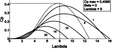
Fig. 2 shows curves for different of the studied 1.5 MW wind turbine.

Fig. 2. curves forβ=0,1,5,10,15 and 20. Doted line corresponds to

β=0 where 0.4096 is achieved.

In Table I aerodynamic design constants can be found, as well as parameters needed for the drawing of Fig. 2 curves.

TABLE I. WIND TURBINE AERODYNAMIC PARAMETERS

β = 0, 1, 5, 10, 15 y 20 c1 = 0.4654

c2 = 116

c3 = 0.4

c4 = 5

c5 = 20.24

c6 = 0.08

c7 = 0.035

λ = 0 to 16

B. Gearbox

The gearbox is the mechanical element that multiplies rotational speed of the mechanical turbine into the speed needed for the electric generator . This generation rotational speed is generally slightly faster than the synchronous speed . For the Mexican grid that works at a

60 Hz frequency, = 2π(60 Hz) = 376.99 rad ≈ 377 rad. Thus, electric generator rotational speed is:

(5) Where n is a multiplicative factor and ω is the mechanical turbine (low speed rotor) angular velocity.

The mechanical power delivered at the output of an ideal gearbox as the one considered in this paper is the same as the one extracted from wind and multiplied by the power coefficient , , . For wind at standard conditions (101.3 kPa y 273 K) density value is

0.647 ⁄ , thus:

(7) Where is mechanical torque and is angular speed, both at the fast rotational side of the gearbox (rotational speed of the electrical generator).

C. Electrical generator

For this paper a squirrel cage induction generator was selected given that this type of generator is the most commonly used.

The squirrel cage induction generator model (Asynchronous machine) was obtained from Simulink MatLab®_.

The mechanical turbine inertia constant was added with the electrical generator own inertia, taking into account that this constant is generally ten times bigger in comparison with the generators’ [9].

D. Implementation of wind turbine model

The complete wind turbine model was implemented in

Simulink of MatLab®_{. The mechanical turbine was}

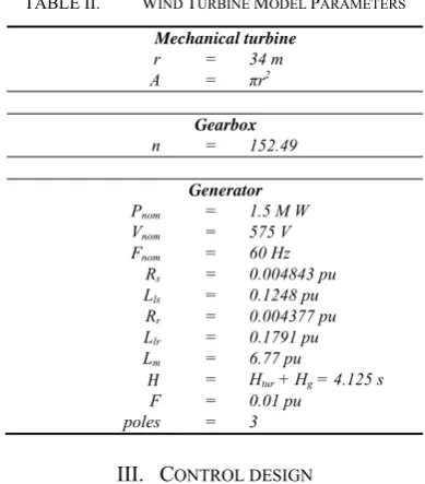
constructed with (3), (4) and (6). The gearbox was modeled as a simple speed gain as in (5). Input to the implemented model is wind speed incident to the mechanical turbine. Model’s output is generated electrical power by the squirrel cage induction generator model. Parameters for the 1.5 MW wind turbine can be found in Table II.

TABLE II. WIND TURBINE MODEL PARAMETERS

Mechanical turbine

r = 34 m A = πr2

Gearbox

n = 152.49

Generator

Pnom = 1.5 M W

Vnom = 575 V

Fnom = 60 Hz

Rs = 0.004843 pu

Lls = 0.1248 pu

Rr = 0.004377 pu

Llr = 0.1791 pu

Lm = 6.77 pu

= Htur + Hg = 4.125 s

F = 0.01 pu poles = 3

III. CONTROL DESIGN

The most common way of controlling a wind turbine consists in varying attack angle at the blades (pitch control) in order to modify the mechanical turbine aerodynamic characteristics and thus modify its performance in accordance to changing wind speed. The blade can be pitched with two methodologies: pitching to stall or pitching to feather. The selection of one or other method has important effects in the wind turbine aerodynamic characteristics. With the pitching to stall method, pitch control is achieved with small negative angle adjustments. The problematic with this methodology is due to undesirable damping and fatigue effects that cannot be effectively modeled. Pitching to feather is the preferred methodology due to the form the wind surrounds the blade.

This aerodynamic effect can be easily modeled and as a consequence, mechanical stress can be foreseen with more reliability. The problem with this type of pitch control is that much bigger angles are needed to effectively control the wind turbine, in this case positive [6]. For the present work, pitching to feather methodology was chosen as can be observed in the positive angles in Table I.

A. Proportional integral controller

A Proportional – Integral (PI) control is a special case of the classic controller family known as Proportional – Integral – Derivative (PID). These types of controllers are up to date the most common way of controlling industry processes in a feedback configuration. More than 95% of all installed controllers are PID [10, 11].

For the designed PI controller for the 1.5 MW horizontal axis wind turbine error signal was selected as:

(8) Where P is the desired output power or set point for the wind turbine, in this case 1.5 MW, and P is the actual delivered power from the wind turbine [6].

The PI control was optimized to achieve rapid response to different wind speed changes and to deliver nominal power output for nominal wind speed (11.75 m/s) as well as higher wind speeds. An open loop analysis was performed at an operating mode for nominal wind speed and without altered aerodynamic blade pitch conditions (v = 11.75 m/s, β = 0º). The Ziegler – Nichols tuning method was then applied to obtain initial gains, which were modified on a trial and error basis to obtain a desirable response. Obtained gains were:

K 0.934 and T 0. 4. Due to the big input signal to the controller, the error was divided by a 10 factor and the integral action saturated at a 45 lower level and a 0 upper level.

B. Fuzzy logic controller

A Fuzzy Logic Controller (FLC) is basically designed by selecting its inputs and outputs, choosing the preprocessing needed for the inputs and de post – processing needed for the outputs, as well as designing each of its four basic components: fuzification, rule – base, inference mechanism

and defuzification. An FLC is an artificial decision making system that operates in closed loop and real time as can be observed in Fig. 3. A more detailed explanation of this methodology can be found in [4 and 12].

For the proposed FLC, inputs to the controller are wind speed v(t) and an e(t) signal as the one in (8). The closed loop diagram for the proposed FLC is shown in Fig. 3.

Fig. 3. Feedback control closed loop for the FLC. Showing inputs and control output.

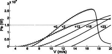
purpose are the P v, which show generated electric power versus wind velocity at constant chosen β angles. Fig. 4 shows some of these curves.

The P v curves were drawn for chosen β =0, 2, 12, 18 y 23. From the curves it is obvious how β angle should be increased in order to maintain a 1.5 MW power generation. Additionally to nominal value power extraction it is also important to obtain maximum generation at low wind speeds.

Fig. 4. Pe – v curves for β =0, 2, 12, 18 and 23. Optimum βangle for current wind speed can be obtained at the intersection with the 1.5 MW doted line.

From Fig. 4 we can observe that for wind speeds below

8 m s⁄ , ideal angle for maximum power extraction is β = 2º. This is an interesting fact because most fixed speed wind turbines maintain a β =0º for speeds below the nominal wind speed. Rules can be derived from observation of these performance curves. Rules loaded to the designed FLC can be found in Table III.

Inference mechanism is basically defined with membership functions which are used to determine the relevance of the set of rules of Table III. Implemented membership functions are shown in Fig. 9, 10 and 11, v(t)

and e(t) inputs and β(t) output respectively. Methods for implication and aggregation where defined as minimum and

maximum respectively. Defuzification process was selected as centroid [4].

C. Fuzzy Proportional Integral controller

The designed Fuzzy Proportional Integral (Fuzzy-PI) controller is a hybrid controller that utilizes two sets of PI

TABLE III. FLC SET OF RULES

v (m/s)

Power e(t)

NegVB NegB Accept PosB PosVB

5 0 1 2 2 2

7 0 1 2 2 2

9 2 2 1 1 0

11 1 0 0 0 0

11.7 1 0 0 0 0

12.6 6 2 1 0 0

13.8 10 6 2 1 0

14.8 14 10 6 2 1

15.5 18 14 10 6 2

16.5 20 18 14 10 6

17.8 20 20 18 14 10

18.6 22 22 20 18 14

19.5 24 24 22 20 18

20.5 24 24 24 22 20

gains in order to achieve a non-linear response. The switching in this controller is achieved with a fuzzy logic section that depends on the input . The PI gains utilize as in (8). Fig. 8 shows a diagram of the proposed Fuzzy-PI controller.

For the proposed Fuzzy-PI algorithm, the fuzzy logic section was designed to smoothly switch between low speed PI gains and nominal and faster wind speed PI gains. The switching was performed following a heuristic approach based in analyzing optimum β angles for different wind speeds from Fig. 4. Following this reasoning the appropriate set of rules was constructed. These rules can be found on Table IV.

Fig. 8. Fuzzy PI controller diagram. Input to fuzzy logic section is wind speed, outputs are PI gains. Input to PI section is error signal, output is control β(t).

TABLE IV. FUZZY LOGIC SECTION SET OF RULES

LWS LSKp LSTi FWS FSKp FSTi

Fig. 5. v(t) FLC input membersip functions.

Fig. 6. e(t) FLC input membersip functions. NegVB, NegB, Accept, PosB and PosVB from left to right.

From Table IV, left column is fuzzy input wind speed v, with two levels, LWS, low wind speed and FWS, high wind speed. Columns to the right are fuzzy outputs K and T, which have two levels as well. LSKp, low speed K , FSKp, fast speed K , LSTi, low speed T, FSTi, fast speed T.

In order to obtain the appropriate PI gains for nominal (11.75 m/s) wind speed and lower than nominal wind speeds the same methodology as in PI control section was used. For lower than nominal wind speed tuning was achieved with the same 1.5 MW set point (v = 6 m/s, β = 2). Obtained gains for low wind speed operation were: K 0.15 and

T 20.

Implemented membership functions are shown in Fig. 9, 10 and 11, v t input, K t and T t outputs respectively. Methods for implication, aggregation and defuzification process where defined as in the FLC.

Fig. 9. Fuzzy logic section input wind speed v. LWS fuzzy set at left and

FWS fuzzy set at right.

Fig. 10. Fuzzy logic section output proportional gain K . FSKp fuzzy set at left and LSKp fuzzy set at right.

Fig. 11. Fuzzy logic section output integral gain 1/ . LSTi fuzzy set at left and FSTi fuzzy set at right.

IV. SIMULATION AND RESULTS

For simulation purposes, wind signal was constructed with two different profiles for a 300 s period. Fig. 12 and 13 show these wind profiles, which correspond to near nominal and faster wind speed operation and low speed operation respectively. For the robustness test noise was added to the wind profiles in Fig. 12 and 13. Fig. 14 and 15. show noisy wind profiles.

Control responses were obtained for both wind speed operation signals (Fig. 12 and 13). Fig. 16, 17, 18 and 19 show power extraction and control signal results.

Fig. 12. Near nominal wind speed operation v(t) signal.

Fig. 13. Low wind speed operation v(t) signal.

Fig. 14. Near nominal wind speed operation, noisy v(t) signal.

Fig. 15. Low wind speed operation, noisy v(t) signal.

From Fig. 16 it can be seen how all control algorithms obtain adequate power control at nominal 1.5 MW level. However, low β angles (Fig. 17) present at the FLC and Fuzzy-PI algorithms achieve better performance for low wind speeds.

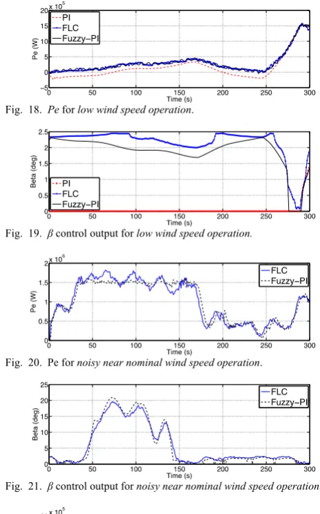
Fig. 18 clearly shows how FLC and Fuzzy PI algorithms performance surpass PI control algorithm performance for low wind speeds. Maximum power extractions for FLC and Fuzzy-PI are due to small β angles near 2º as can be observed from Fig. 19.

Fig. 18, 19, 20 and 21 show results for extracted power and control signal for noisy wind speed input (Fig. 13 and 14) to controllers for FLC and Fuzzy-PI methodologies.

From Fig. 20 it can be seen how FLC has no adequate power control at nominal 1.5 MW level because of its dependence on wind speed input to operate. However, Fuzzy-PI algorithm responds in an adequate form. This can also be observed at Fig. 21 where control signal for the FLC methodology is affected by noise.

These same results can be observed in Fig. 23 for lower than nominal wind speeds. However, Fig. 22 shows no clear advantage between FLC and Fuzzy-PI controller.

Fig. 16. Pe for near nominal wind speed operation.

0 5 10.25 15 20 25

0 0.5 1

wind speed (m/s)

per

ti

nence

9.5 11

0 50 100 150 200 250 300

5 7.5 10 12.5 15 17.5 20

Time (s)

V (m/

s

)

0 50 100 150 200 250 300

0 10 20x 10

5

Time (s)

Pe

(

W

)

0 50 100 150 200 250 300

5 10 15 20

Time (s)

V (m

/s)

0 50 100 150 200 250 300

0 5 10

Time (s)

V (m

Fig. 17. β control output for near nominal wind speed operation.

Fig. 18. Pe for low wind speed operation.

Fig. 19. β control output for low wind speed operation.

Fig. 20. Pe for noisy near nominal wind speed operation.

Fig. 21. β control output for noisynear nominal wind speed operation.

Fig. 22. Pe for noisylow wind speed operation.

Fig. 23. β control output for noisylow wind speed operation.

V. CONCLUSION

Research presents a PI, FLC and PI control comparison in simulation for a 1.5 MW horizontal axis fixed speed wind turbine model, PI control algorithm achieves good performance for power extraction near the nominal 1.5 MW

for nominal wind speeds (around 11.75 m/s) and higher speeds, however, a constant 0º β angle at lower speeds results in poor power extraction. The implemented FLC and Fuzzy-PI control algorithms surpass the traditional PI thanks to its inherent characteristics to deal directly with non linear models. From quick inspection to power versus wind extraction performance curves all needed control rules can be extracted. A fuzzy logic section in the Fuzzy-PI algorithm allows for a non linear operation using a smooth PI gain switching methodology with good results. A robustness test was performed by adding a noisy wind speed signal to the FLC and Fuzzy-PI control algorithms. Results demonstrate the inherent ability of the Fuzzy-PI control algorithm to deal with this kind of noise. FLC algorithm shows no adequate response for noisy , which is understandable because of its dependence in this control input signal. These results are important because in a real scenario wind speed measurement is a difficult task.

REFERENCES

[1] L. A. Barroso, H. Rudnick, F. Sensfuss and P. Linares, “The Green Effect” in IEEE Power & Energy, vol. 8, num. 5, IEEE PES, EUA, 2010, pp. 22-35.

[2] J. Anzurez-Marin, L. A. Torres-Salomao and I. I. Lázaro-Castillo, “Fuzzy Logic Control for a Two Tanks Hydraulic System Model”, in

Proc. 2011 IEEE Electronics, Robotics and Automotive Mechanics Conference CERMA 2011, Cuernavaca, Mexico, 2011.

[3] S.K. Hong, and Y. Nam, “An LMI-Based Fuzzy Sate Feedback Control with Multi-Objectives”, KSME International Journal, Springer, Korea, 2003, pp. 105-113.

[4] Passino, K.M., and S. Yurkovich, Fuzzy Control, Addison-Wesley, United States of America, 1998.

[5] L. A. Torres-Salomao and H. Gámez-Cuatzin, “Fuzzy Logic Control and PI control Comparison for a 1.5 MW Horizontal Axis Wind Turbine”, 2012 16th _{International Conference on System Theory,}

Control and Computing, ICSTCC, Control Society, Sinaia, Romania. [6] Burton T., Sharpe D., Jenkins N. and Bossanyi E., Wind Energy

Handbook, Wiley, England, 2001.

[7] Johnson G. L., Wind Energy Systems, Electronic edition, USA, 2006. [8] R. Kyoungsoo and H. Choi, “Application of neural network controller

for maximum power extraction of a grid-connected wind turbine”, Springer – Verlag, 2004.

[9] Z. Saad-Saoud and N. Jenkins, “Simple wind farm dynamic model”, in IEEE Proc. Gener. Transm. Distrib., Vol. 142, No. 5, 1995, pp. 545-548.

[10] K.J. Åström and T.H. Hägglund, “New tuning methods for PID controllers”, Proceedings of the 3rd European Control Conference, 1995, p.2456–62.

[11] I.I. Lázaro-Castillo, Ingeniería de Sistemas de Control Continuo, UMSNH, COECyT Michoacán, FIE, Mexico, 2008.