Word Sense Disambiguation
Deniz Yuret
∗ Koc¸ UniversityMehmet Ali Yatbaz
Koc¸ UniversityWe introduce a generative probabilistic model, the noisy channel model, for unsupervised word sense disambiguation. In our model, each context C is modeled as a distinct channel through which the speaker intends to transmit a particular meaning S using a possibly ambiguous word W. To reconstruct the intended meaning the hearer uses the distribution of possible meanings in the given context P(S|C) and possible words that can express each meaning P(W|S). We assume P(W|S)is independent of the context and estimate it using WordNet sense frequencies. The main problem of unsupervised WSD is estimating context-dependent P(S|C)without access to any sense-tagged text. We show one way to solve this problem using a statistical language model based on large amounts of untagged text. Our model uses coarse-grained semantic classes for S internally and we explore the effect of using different levels of granularity on WSD per-formance. The system outputs fine-grained senses for evaluation, and its performance on noun disambiguation is better than most previously reported unsupervised systems and close to the best supervised systems.
1. Introduction
Word sense disambiguation (WSD) is the task ofidentifying the correct sense ofan ambiguous word in a given context. An accurate WSD system would benefit appli-cations such as machine translation and information retrieval. The most successful WSD systems to date are based on supervised learning and trained on sense-tagged corpora. In this article we present an unsupervised WSD algorithm that can leverage untagged text and can perform at the level of the best supervised systems for the all-nouns disambiguation task.
The main drawback ofthe supervised approach is the difficulty ofacquiring considerable amounts oftraining data, also known as the knowledge acquisition bottleneck. Yarowsky and Florian (2002) report that each successive doubling ofthe training data for WSD only leads to a 3–4% error reduction within their experimental range. Banko and Brill (2001) experiment with the problem ofselection among confusable words and show that the learning curves do not converge even after
∗Koc¸ University, Department ofComputer Engineering, 34450 Sarıyer, ˙Istanbul, Turkey. E-mail: dyuret@ku.edu.tr, myatbaz@ku.edu.tr.
a billion words oftraining data. They suggest unsupervised, semi-supervised, or active learning to take advantage oflarge data sets when labeling is expensive. Yuret (2004) observes that in a supervised naive Bayes WSD system trained on SemCor, approximately halfofthe test instances do not contain any ofthe contextual features (e.g., neighboring content words or local collocation patterns) observed in the training data. SemCor is the largest publicly available corpus ofsense-tagged text, and has only about a quarter million sense-tagged words. In contrast, our unsupervised system uses the Web1T data set (Brants and Franz 2006) for unlabeled examples, which contains counts from a 1012word corpus derived from publicly-available Web pages.
A note on the term “unsupervised” may be appropriate here. In the WSD literature “unsupervised” is typically used to describe systems that do not directly use sense-tagged corpora for training. However, many of these unsupervised systems, including ours, use sense ordering or sense frequencies from WordNet (Fellbaum 1998) or other dictionaries. Thus it might be more appropriate to call them weakly supervised or semi-supervised. More specifically, context–sense pairs or context–word–sense triples are not observed in the training data, but context-word frequencies (from untagged text) and word-sense frequencies (from dictionaries or other sources) are used in model building. One ofthe main problems we explore in this study is the estimation ofcontext-dependent sense probabilities when no context–sense pairs have been observed in the training data.
The first contribution ofthis article is a probabilistic generative model for word sense disambiguation that seamlessly integrates unlabeled text data into the model building process. Our approach is based on the noisy channel model (Shannon 1948), which has been an essential ingredient in fields such as speech recognition and machine translation. In this study we demonstrate that the noisy channel model can also be the key component for unsupervised word sense disambiguation, provided we can solve the context-dependent sense distribution problem. In Section 2.1 we show one way to estimate the context-dependent sense distribution without using any sense-tagged data. Section 2.2 outlines the complete unsupervised WSD algorithm using this model. We estimate the distribution ofcoarse-grained semantic classes rather than fine-grained senses. The solution uses the two distributions for which we do have data: the distribu-tion ofwords used to express a given sense, and the distribudistribu-tion ofwords that appear in a given context. The first can be estimated using WordNet sense frequencies, and the second can be estimated using ann-gram language model as described in Section 2.3.
The second contribution ofthis article is an exploration ofsemantic classes at differ-ent levels of granularity for word sense disambiguation. Using fine-grained senses for model building is inefficient both computationally and from a learning perspective. The noisy channel model can take advantage ofthe close distribution ofsimilar senses ifthey are grouped into semantic classes. We take semantic classes to be groups ofWordNet synsets defined using the hypernym hierarchy. In each experiment we designate a number ofsynsets high in the WordNet hypernym hierarchy as “head synsets” and use their descendants to partition the senses into separate semantic classes. In Section 3 we present performance bounds for such class-based WSD and describe our method of exploring the different levels of granularity.
2. The Noisy Channel Model for WSD
2.1 Model
The noisy channel model has been the foundation of standard models in speech recog-nition (Bahl, Jelinek, and Mercer 1983) and machine translation (Brown et al. 1990). In this article we explore its application to WSD. The noisy channel model can be used whenever a signal received does not uniquely identify the message being sent. Bayes’ Law is used to interpret the ambiguous signal and identify the most probable intended message. In WSD, we model each context as a distinct channel where the intended message is a word sense (or semantic class) S, and the signal received is an ambiguous wordW. In this section we will describe how to model a given contextCas a noisy channel, and in particular how to estimate the context-specific sense distribution without using any sense-tagged data.
Equation (1) expresses the probability ofa senseSofwordWin a given contextC. This is the well-known Bayes’ formula with an extra P(.|C) in each term indicating the dependence on the context.
P(S|W,C)= P(W|S,C)P(S|C)
P(W|C) (1)
To perform WSD we need to find the senseSthat maximizes the probability P(S|W,C). This is equivalent to the maximization ofthe product P(W|S,C)P(S|C) because the denominator P(W|C) does not depend on S. To perform the maximization, the two distributions P(W|S,C) and P(S|C) need to be estimated for each contextC.
The main challenge is to estimate P(S|C), the distribution ofword senses that can be expressed in the given context. In unsupervised WSD we do not have access to any sense-tagged data, thus we do not know what senses are likely to be expressed in any given context. Therefore it is not possible to estimate P(S|C) directly.
What we do have is the word frequencies for each sense P(W|S), and the word frequencies for the given context P(W|C). We use the WordNet sense frequencies to estimate P(W|S) and a statistical language model to estimate P(W|C) as detailed in Section 2.3. We make the independence assumption P(W|S,C)=P(W|S), that is, the distribution ofwords used to express a particular sense is the same for all contexts. Finally, the relationship between the three distributions, P(S|C), P(W|S,C), and P(W|C) is given by the total probability theorem:
P(W|C)=
S
P(S|C)P(W|S,C) (2)
We can solve for P(S|C) using linear algebra. LetWSbe a matrix,sandwtwo vectors such that:
WSij =P(W=i|S=j)
sj=P(S=j|C=k)
Using this new form, we can see that Equation (2) is equivalent to the linear equation
w=WS×sandscan be solved using a linear solver. TypicallyWSis a tall matrix and the system has no exact solutions. We use the Moore–Penrose pseudoinverseWS+to compute an approximate solution:
s=WS+×w (4)
Appendix A discusses possible scaling issues ofthis solution and offers alternative solutions. We use the pseudoinverse solution in all our experiments because it can be computed fast and none of the alternatives we tried made a significant difference in WSD performance.
2.2 Algorithm
Section 2.1 described how to apply the noisy channel model for WSD in a single context. In this section we present the steps we follow in our experiments to simultaneously apply the noisy channel model to all the contexts in a given word sense disambiguation task.
Algorithm 1
1. LetWbe the vocabulary. In this study we took the vocabulary to be the approximately 12,000 nouns in WordNet that have non-zero sense frequencies.
2. LetSbe the set ofsenses or semantic classes to be used. In this study we used various partitions ofnoun synsets as semantic classes.
3. LetCbe the set ofcontexts (nine-word windows for a 5-gram model) surrounding each target word in the given WSD task.
4. Compute the matrixWCwhereWCik=P(W=i|C=k). Hereiranges
over the vocabularyWandkranges over the contextsC. This matrix concatenates the (w) word distribution vectors from Equation (4) for each context. The entries ofthe matrix are computed using then-gram language model described in Section 2.3. This is the most expensive step in the algorithm (see Appendix B for a discussion of implementation efficiency).
5. Compute the matrixWSwhereWSij=P(W=i|S=j). Hereiranges over
the vocabularyWandjranges over the semantic classesS. The entries of the matrix are computed using the WordNet sense frequencies.
6. Compute the matrixSC=WS+×WCwhereSCjk=P(S=j|C=k).
Herejranges over the semantic classesSandkranges over the contextsC. This step computes the pseudoinverse solution described in Section 2.1 simultaneously for all the contexts, and the resultingSCmatrix is a concatenation ofthe (s) solution vectors from Equation (4) for each context.
WS+is the pseudoinverse ofthe matrixWS.
and P(W|S) comes from the row of theWSmatrix that corresponds to the word to be disambiguated.
8. Compute the fine-grained answer for each WSD instance by taking the most frequent (lowest numbered) sense in the chosen semantic class.
9. Apply theone sense per discourseheuristic: Ifa word is found to have multiple senses in a document, replace them with the majority answer.
2.3 Estimation Procedure
In Section 2.1, we showed how the unsupervised WSD problem expressed as a noisy channel model can be decomposed into the estimation oftwo distributions: P(W|S) and P(W|C). In this section we detail our estimation procedure for these two distributions.
To estimate P(W|S), the distribution ofwords that can be used to express a given meaning, we used the WordNet sense frequencies.1We did not perform any smoothing for the zero counts and used the maximum likelihood estimate: count(W,S)/count(S). As described in later sections, we also experimented with grouping similar WordNet senses into semantic classes. In this caseSstands for the semantic class, and the counts from various senses of a word in the same semantic class are added together to estimate P(W|S).
To estimate the distribution ofwords in a given context, P(W|C), we used a 5-gram language model. We define the context as the nine-word window centered on the target
wordw1w2. . .w9, whereW=w5. The probability ofa word in the given context can be
expressed as:
P(W=w5)∝P(w1. . .w9) (5)
=P(w1)P(w2|w1). . .P(w9|w1. . .w8) (6)
∝P(w5|w1. . .w4)P(w6|w2. . .w5)P(w7|w3. . .w6) (7)
P(w8|w4. . .w7)P(w9|w5. . .w8)
Equation (5) indicates that P(W|C) is proportional to P(w1. . .w9) because the other
words in the context are fixed for a given WSD instance. Equation (6) is the standard decomposition ofthe probability ofa word sequence into conditional probabilities. The first four terms do not include the target wordw5, and have been dropped in
Equa-tion (7). We also truncate the remaining condiEqua-tionals to four words reflecting the Markov assumption ofthe 5-gram model. Finally, using an expression that is proportional to P(W|C) instead ofP(W|C) itselfwill not change the WSD result because we are taking the argmax in Equation (1).
Each term on the right hand side ofEquation (7) is estimated using a 5-gram language model. To get accurate domain-independent probability estimates we used the Web 1T data set (Brants and Franz 2006), which contains the counts ofword sequences up to length five in a 1012 word corpus derived from publicly-accessible Web pages. Estimation ofP(W|C) is the most computationally expensive step ofthe algorithm, and some implementation details are given in Appendix B.
Figure 1
Upper bound on fine-grained accuracy for a given number of semantic classes.
3. Semantic Classes
Our algorithm internally differentiates semantic classes rather than fine-grained senses. Using fine-grained senses in the noisy channel model would be computationally ex-pensive because the word–sense matrix needs to be inverted (see Equation [4]). It is also unclear whether using fine-grained senses for model building will lead to better learning performance: The similarity between the distributions of related senses is ignored and the data becomes unnecessarily fragmented.
Even though we use coarse-grained semantic classes for model building, we use fine-grained senses for evaluation. During evaluation, the coarse-grained semantic classes predicted by the model are mapped to fine-grained senses by picking the lowest numbered WordNet sense in the chosen semantic class.2This is necessary to perform a meaningful comparison with published results.
We take semantic classes to be groups ofWordNet synsets defined using the hyper-nym hierarchy (see Section 6 for alternative definitions). Section 4 presents three WSD experiments using different sets of semantic classes at different levels of granularity. In each experiment we designate a number ofsynsets high in the WordNet hypernym hierarchy as “head synsets” and use their descendants to form the separate semantic classes.
An arbitrary set ofhead synsets will not necessarily have mutually exclusive and collectively exhaustive descendants. To assign every synset to a unique semantic class, we impose an ordering on the semantic classes. Each synset is assigned only to the first semantic class whose head it is a descendant ofaccording to this ordering. Ifthere are synsets that are not descendants ofany ofthe heads, they are collected into a separate semantic class created for that purpose.
Using the coarse-grained semantic classes for prediction, Algorithm 1 will be unable to return the correct fine-grained sense when this is not the lowest numbered sense in a semantic class. To quantify the restrictive effect of working with a small number of semantic classes, Figure 1 plots the number ofsemantic classes versus the best possible
oracle accuracy for the nouns in the SemCor corpus. To compute the oracle accuracy, we assume that the program can find the correct semantic class for each instance, but has to pick the first sense in that class as the answer. To construct a given number ofsemantic classes, we used the following algorithm:
Algorithm 2
1. Initialize all synsets to be in a single “default” semantic class.
2. For each synset, compute the following score: the oracle accuracy achieved ifthat synset and all its descendants are split into a new semantic class.
3. Take the synset with the highest score and split that synset and its descendants into a new semantic class.
4. Repeat steps 2 and 3 until the desired number ofsemantic classes is achieved.
The upper bound on fine-grained accuracy given a small number ofsemantic classes is surprisingly high. In particular, the best reported noun WSD accuracy (78%) is achievable ifwe could perfectly distinguish between five semantic classes.
4. Three Experiments
We ran three experiments with the noisy channel model using different sets of semantic classes. The first experiment uses the 25 WordNet semantic categories for nouns, the second experiment looks at what happens when we group all the senses to just two or three semantic classes, and the final experiment optimizes the number ofsemantic classes using one data set (which gives 135 classes) and reports the out-of-sample result using another data set.
The noun instances from the last three SensEval/SemEval English all-words tasks are used for evaluation. We focus on the disambiguation of nouns for several reasons. Nouns constitute the largest portion ofcontent words (48% ofthe content words in the Brown corpus [Kucera and Francis 1967] are nouns). For many tasks and applications (e.g., Web queries [Jansen, Spink, and Pfaff 2000]) nouns are the most frequently encoun-tered and important part ofspeech. Finally, WordNet has a more complete coverage ofnoun semantic relations than other parts ofspeech, which is important for our experiments with semantic classes.
As described in Section 2.2 we use the model to assign each ambiguous word to its most likely semantic class in all the experiments. The lowest numbered sense in that class is taken as the fine-grained answer. Finally we apply theone sense per discourse
heuristic: Ifthe same word has been assigned more than one sense within the same document, we take a majority vote and use sense numbers to break the ties.
Table 1
Baselines for the three SensEval English all-words tasks; the WordNet version used (WN); number ofnoun instances (Nouns); percentage accuracy ofthe first-sense baseline (FSB); the top three supervised systems; and the best unsupervised system (Unsup). The last row gives the total score ofthe best systems on the three tasks.
Task WN Nouns FSB 1st 2nd 3rd Unsup
senseval2 1.7 1,067 71.9 78.0 74.5 70.0 61.8 senseval3 1.7.1 892 71.0 72.0 71.2 71.0 62.6 semeval07 2.1 159 64.2 68.6 66.7 66.7 63.5
total 2,118 70.9 74.4 72.5 70.2 62.2
unsupervised system is given in the last column. The reported unsupervised systems do use the sense ordering and frequency information from WordNet.
4.1 First Experiment: The 25 WordNet Categories
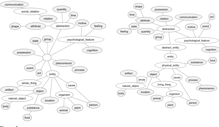
In previous work, descendants of25 special WordNet synsets (known as the unique beginners) have been used as the coarse-grained semantic classes for nouns (Crestan, El-B`eze, and De Loupy 2001; Kohomban and Lee 2005). These unique beginners were used to organize the nouns into 25 lexicographer files based on their semantic category during WordNet development. Figure 2 shows the synsets at the top ofthe noun hierarchy in WordNet. The 25 unique beginners have been shaded, and the two graphics show how the hierarchy evolved between the two WordNet versions used in this study.
Figure 2
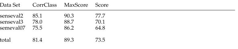
[image:8.486.51.432.411.632.2]Table 2
The performance of the noisy channel model with the 25 semantic classes based on WordNet lexicographer files. The columns give the data set, the percentage oftimes the model picks the correct semantic class, maximum possible fine-grained score ifthe model had always picked the correct class, and the actual score.
Data Set CorrClass MaxScore Score
senseval2 85.1 90.3 77.7
senseval3 78.0 88.7 70.1
semeval07 75.5 86.2 64.8
total 81.4 89.3 73.5
We ran our initial experiments using these 25 WordNet categories as semantic classes. The distribution ofwords for each semantic class, P(W|S), is estimated based on WordNet sense frequencies. The distribution of words for each context, P(W|C), is estimated using a 5-gram model based on the Web 1T corpus. The system first finds the most likely semantic class based on the noisy channel model, then picks the first sense in that class. Table 2 gives the results for the three data sets, which are significantly higher than the previously reported unsupervised results.
[image:9.486.55.400.460.659.2]To illustrate which semantic classes are the most difficult to disambiguate, Table 3 gives the confusion matrix for the Senseval2 data set. We can see that frequently occur-ring concrete classes like person and body are disambiguated well. The largest source oferrors are the abstract classes like act,attribute,cognition, andcommunication. These 25 classes may not be the ideal candidates for word sense disambiguation. Even though they allow a sufficient degree of fine-grained distinction (Table 2 shows that we can get
Table 3
Confusion matrix for Senseval2 data with the 25 WordNet noun classes. The rows are actual classes, the columns are predicted classes. Column names have been abbreviated to save space. The last two columns give the frequency of the class (F) and the accuracy of the class (A).
ac an ar at bo co co ev fe fo gr lo mo ob pe ph po pr qu re sh st su ti F A act 58 0 4 7 0 7 2 3 2 0 5 0 0 0 0 0 14 110 2 0 0 9.159.8 animal 0 17 5 0 0 0 0 0 0 0 0 0 0 0 0 0 0 0 0 0 0 0 0 0 2.1 77.3 artifact 0 0 66 2 0 0 6 5 0 0 5 10 10 0 0 0 0 0 3 10 0 8.4 73.3 attribute 3 0 0 19 0 3 0 0 0 0 0 10 12 0 2 10 0 13 0 0 3.4 52.8 body 0 0 0 0 123 0 0 0 0 0 0 0 0 0 0 0 0 0 1 0 0 0 0 0 11.6 99.2 cognition 6 0 12 0 82 5 10 0 0 2 1110 10 5 10 5 0 0 10.7 71.9 communicat 2 0 10 0 2 29 10 0 0 2 5 0 0 10 0 0 10 0 0 2 4.3 63.0 event 0 0 0 0 0 0 0 19 0 0 0 0 0 0 0 1 0 0 0 0 0 0 0 1 2.0 90.5 feeling 0 0 0 0 0 0 0 0 4 0 0 0 0 0 0 0 0 0 0 0 0 0 0 0 0.4 100.
food 0 0 0 0 0 0 0 0 0 10 0 0 0 0 0 0 0 0 0 0 0 0 0 0.1100. group 0 0 0 2 0 5 0 0 0 0 69 2 0 3 0 0 0 0 0 110 0 17.9 82.1 location 0 0 0 10 0 0 0 0 0 0 22 0 0 0 0 0 0 0 0 0 0 0 0 2.2 95.7
motive 0 0 0 0 0 0 10 0 0 0 0 10 0 0 0 0 0 0 0 0 0 0 0.2 50.0 object 2 0 0 0 0 0 0 0 0 0 0 1110 0 0 0 10 0 0 0 10.7 14.3 person 2 4 0 0 0 110 0 0 10 0 0 168 0 0 0 0 0 0 0 0 0 16.6 94.9 phenomenon 10 0 10 10 2 0 0 0 0 0 0 0 3 0 0 0 3 0 0 0 0 1.0 27.3 possession 0 0 0 0 0 0 0 0 0 0 0 0 0 0 0 0 4 0 0 0 0 0 0 0 0.4 100.
process 0 0 0 0 0 0 0 2 0 0 0 0 0 0 0 0 0 12 0 0 0 1 0 0 1.4 80.0 quantity 0 0 0 10 0 0 10 0 10 0 0 0 0 0 0 10 0 0 0 0 0 1.2 76.9 relation 10 0 0 0 0 0 0 0 0 0 0 0 0 0 0 0 0 0 2 0 0 0 0 0.3 66.7 shape 0 0 0 0 0 0 0 0 0 0 0 0 0 0 0 0 0 0 0 0 10 0 0 0.1100. state 10 15 0 112 0 0 10 0 0 10 0 0 0 0 0 98 0 0 10.4 88.3 substance 0 0 0 0 0 0 0 0 0 0 0 0 0 0 0 0 0 0 0 0 0 0 10 0 0.9 100.
Table 4
The performance of the noisy channel model with two to three semantic classes. The columns give the data set, the head synsets, the percentage oftimes the model picks the correct semantic class, maximum possible fine-grained score ifthe model had always picked the correct class, and the actual score.
Data Set Heads CorrClass MaxScore Score
senseval2 entity/default 86.6 76.8 74.9
senseval3 entity/default 94.2 75.8 71.2
senseval3 object/entity/default 93.8 77.4 72.9
semeval07 psychological-feature/default 91.2 74.8 68.6
85–90% ifwe could pick the right class every time), they seem too easy to confuse. In the next few experiments we will use these observations to design better sets of semantic classes.
4.2 Second Experiment: Distinguishing Mental and Physical Concepts
Figure 1 shows that the upper bound for fine-grained disambiguation is relatively high even for a very small number of semantic classes. In our next experiment we look at how well our approach can perform differentiating only two or three semantic classes.
We use Algorithm 2 applied to the appropriate version ofSemCor to pick the head synsets used to define the semantic classes. Figure 2 shows that the top level ofthe hypernym hierarchy has changed significantly between the WordNet versions. Thus, different head synsets are chosen for different data sets. However, the main distinction captured by our semantic classes seems to be between mental and physical concepts. Table 4 gives the results. The performance with a few semantic classes is comparable to the top supervised algorithms in each ofthe three data sets.
4.3 Third Experiment: Tuning the Number of Classes
Increasing the number of semantic classes has two opposite effects on WSD perfor-mance. The higher the number, the finer distinctions we can make, and the maximum possible fine-grained accuracy goes up. However, the more semantic classes we define, the more difficult it becomes to distinguish them from one another. For an empirical analysis ofthe effect ofsemantic class granularity on the fine-grained WSD accuracy, we generated different sets of semantic classes using the following algorithm.
Algorithm 3
1. Sort all the synsets according to their “subtree frequency”: i.e., the total frequency of each synset’s descendants in the hypernym tree.
2. Take the desired number ofsynsets with the highest subtree frequency and use them as head synsets, that is, split their descendants into separate semantic classes.
Figure 3
The fine-grained accuracy on Senseval2 data set for a given number of semantic classes.
Figure 1 gives the best possible oracle accuracy, Figure 3 gives the actual WSD accuracy; (ii) Algorithm 2 chooses the head synsets based on their oracle score, Algorithm 3 chooses them based on their subtree frequency.
As we suspected, the relationship is not simple or monotonic. However, one can identify distinct peaks at 3, 25, and 100–150 semantic classes. One hypothesis is that these peaks correspond to “natural classes” at different levels of granularity. Here are some example semantic classes from each peak:
3 classes entity, abstraction
25 classes action, state, content, location, attribute, ...
135 classes food, day, container, home, word, business, feeling, material, job, man, ...
To test the out-of-sample effect of tuning the semantic classes based on the peaks ofFigure 3, we used the SemEval-2007 data set as our test sample. When the 135 semantic classes from the highest peak are used for the disambiguation of the nouns in the SemEval-2007 data set, an accuracy of69.8% was achieved. This is higher than the accuracy ofthe best supervised system on this task (68.6%), although the difference is not statistically significant.
5. Discussion
In this section we will address several questions raised by the results ofthe experi-ments. Why do we get different results from different data sets? Are the best results significantly different than the first-sense baseline? Can we improve our results using better semantic classes?
5.1 Why Do We Get Different Results from Different Data Sets?
Table 5
Result summary for the three data sets. The columns give the data set, the results of the three experiments, best reported result, the first-sense baseline, and the number ofinstances.
Data set Exp1 Exp2 Exp3 Best FSB Instances
senseval2 77.7 74.9 - 78.0 71.9 1,067
senseval3 70.1 72.9 - 72.0 71.0 892
semeval07 64.8 68.6 69.8 68.6 64.2 159
The SemEval-2007 data set appears to be significantly different from the other two with its generally lower baseline and scores. The difference in accuracy is probably due to the difference in data preparation. In the two Senseval data sets all content words were targeted for disambiguation. In the SemEval-2007 data set only verbs and their noun arguments were selected, targeting only about 465 lemmas from about 3,500 words oftext. For the Senseval-3 data set none ofour results, or any published result we know of, is significantly above the baseline for noun disambiguation. This may be due to extra noise in the data—the inter-annotator agreement for nouns in this data set was 74.9%.
5.2 Are the Best Results Significantly Different Than the FSB?
Among all the published results for these three data sets, our two results for the Senseval-2 data set and the top supervised result for the Senseval-2 data set are the only ones statistically significantly above the FSB for noun disambiguation at the 95% confidence interval. This is partly because ofthe lack ofsufficient data. For example, the SemEval-2007 data set has only 159 nouns; and a result of71.8% would be needed to demonstrate a difference from the baseline of 64.2% at the 95% confidence interval.
More importantly, however, statistical significance should not be confused with “significance” in general. A statistically significant difference may not be necessary or sufficient for a significant impact on an application. Even a WSD system that is statis-tically indistinguishable from the baseline according to the “total accuracy” metric is most probably providing significantly different answers compared to always guessing the first sense. There are metrics that can reveal these differences, such as “balanced error rate” (i.e., arithmetic average of the error rates for different senses) or “accuracy in detecting the use ofa non-dominant sense.”
Finally, the relatively high first-sense baseline (e.g., 71.0% for Senseval-3 nouns) combined with the relatively low inter-annotator agreement (e.g., 74.9% for Senseval-3 nouns) makes progress in the traditional WSD task difficult. Annotators who are perfectly proficient in comprehending language nevertheless find it difficult to distin-guish between artificially-created dictionary senses. Ifour long term goal is to model human competence in language comprehension, it would make sense to focus on tasks at which humans are naturally competent. Dictionary-independent tasks such as lexical substitution or textual entailment may be the right steps in this direction.
5.3 Can We Improve Our Results Using Better Semantic Classes?
Table 6
The performance ofthe noisy channel model with the best set ofsemantic classes picked for each data set. The columns give the data set, the number ofclasses, maximum possible score ifthe model always picks the correct class, percentage oftimes it actually picks the correct class, and its fine-grained accuracy.
Data Set NumClass MaxScore CorrClass Score
senseval2 23 89.2 88.8 80.1
senseval3 29 87.2 87.4 77.4
semeval07 12 84.9 89.9 79.2
Algorithm 4
1. Initialize all synsets to be in a single “default” semantic class.
2. For each synset, compute the following score: the WSD accuracy achieved ifthat synset and all its descendants are split into a new semantic class.
3. Take the synset with the highest score and split that synset and its descendants into a new semantic class.
4. Repeat steps 2 and 3 until the WSD accuracy can no longer be improved.
Algorithm 4 was run for each of the three data sets, which resulted in three different sets ofsemantic classes. The noisy channel model was applied with the best set of semantic classes for each data set. Table 6 summarizes the results. Note that these results are not predictive ofout-of-sample accuracy because Algorithm 4 picks a specific set of semantic classes optimal for a given data set. But the results do indicate that a better set ofsemantic classes may lead to significantly better WSD accuracy. In particular each result in Table 6 is significantly higher than previously reported supervised or unsupervised results.
How to construct a good set ofsemantic classes that balance specificity and identi-fiability is a topic ofongoing research. See Kohomban and Lee (2007) for a supervised solution using feature-based clustering that tries to maintain feature–class coherence. Non-parametric Bayesian approaches such as Teh et al. (2006) applied to context distri-butions could reveal latent senses in an unsupervised setting.
6. Related Work
For a general overview ofdifferent approaches to WSD, see Navigli (2009) and Stevenson (2003). The Senseval and SemEval workshops (Cotton et al. 2001; Mihalcea and Edmonds 2004; Agirre, M `arquez, and Wicentowski 2007) are good sources ofrecent work, and have been used in this article to benchmark our results.
Using statistical language models based on large corpora for WSD has been ex-plored in Yuret (2007) and Hawker (2007). For specific modeling techniques used in this article see Yuret (2008); for a more general review of statistical language modeling see Chen and Goodman (1999), Rosenfeld (2000), and Goodman (2001).
Grouping similar senses into semantic classes for WSD has been explored in previ-ous work. Senses that are similar have been identified using WordNet relations (Peters, Peters, and Vossen 1998; Crestan, El-B`eze, and De Loupy 2001; Kohomban and Lee 2005), discourse domains (Magnini et al. 2003), annotator disagreements (Chklovski and Mihalcea 2003), and other lexical resources such as Roget (Yarowsky 1992), LDOCE (Dolan 1994), and ODE (Navigli 2006).
Ciaramita and Altun (2006) build a supervised HMM tagger using “supersenses,” essentially the 25 WordNet noun categories we have used in our first experiment in addition to 15 verb categories similarly defined. They report a supersense precision of 67.60 for nouns and verbs of Senseval-3. Table 2 gives our supersense score as 78% for Senseval-3 nouns. However, the results are not directly comparable because they do not report the noun and verb scores separately or calculate the corresponding fine-grained score to compare with other Senseval-3 results.
Kohomban and Lee (2007) go beyond the WordNet categories based on lexicogra-pher files and experiment with clustering techniques to construct their semantic classes. Their classes are based on local features from sense-labeled data and optimize feature– class coherence rather than adhering to the WordNet hierarchy. Their supervised system achieves an accuracy of74.7% on Senseval-2 nouns and 73.6% on Senseval-3 nouns.
The systems mentioned so far are supervised WSD systems. Agirre and Martinez (2004) explore the large-scale acquisition ofsense-tagged examples from the Web and train supervised, minimally supervised (requiring sense bias information from hand-tagged corpora, similar to our system), and fully unsupervised WSD algorithms using this corpus. They report good results on the Senseval-2 lexical sample data compared to other unsupervised systems. Martinez, de Lacalle, and Agirre (2008) test a similar set of systems trained using automatically acquired corpora on Senseval-3 nouns. Their mini-mally supervised system obtains 63.9% accuracy on polysemous nouns from Senseval-3 (corresponding to 71.86% on all nouns).
7. Contributions
We have introduced a new generative probabilistic model based on the noisy channel framework for unsupervised word sense disambiguation. The main contribution of this model is the reduction ofthe word sense disambiguation problem to the estimation of two distributions: the distribution ofwords used to express a given sense, and the dis-tribution ofwords that appear in a given context. In this framework, context similarity is determined by the distribution ofwords that can be placed in the given context. This replaces the ad hoc contextual feature design process by a statistical language model, allowing the advances in language modeling and the availability oflarge unlabeled corpora to have a direct impact on WSD performance.
the relationship between granularity and fine-grained accuracy is complex, thus more work is needed to determine an ideal set ofsemantic classes.
In several experiments we compare the performance of our unsupervised WSD system with the best systems from previous Senseval and SemEval workshops. We consistently outperform any previously reported unsupervised results and achieve comparable performance to the best supervised results.
Appendix A: Solutions for P(S|C)
To solve for P(S|C) using P(W|C) and P(W|S), we represent the first two as vectors:sj=
P(S=j|C=k) and wi=P(W=i|C=k), and the last one as a matrix: WSij=P(W=
i|S=j). Our problem becomes finding a solution to the linear equation w=WS×s. Using the Moore–Penrose pseudoinverse,WS+, we find a solutions=WS+×w. This solution minimizes the distance|WS×s−w|. There are two potential problems with this pseudoinverse solution. First, it may violate the non-negativity and normalization constraints ofa probability distribution. Second, a maximum likelihood estimate should minimize the cross entropy between WS×s and w, not the Euclidean distance. We addressed the normalization problem using a constrained linear solver and the cross-entropy problem using numerical optimization. However, our experiments showed the difference in WSD performance to be less than 1% in each case. The pseudoinverse solution, s=WS+×w, can be computed quickly and works well in practice, so this is the solution that is used in all our experiments.
Appendix B: Estimating P(W|C)
Estimating P(W|C) for each context is expensive because the number of words that need to be considered is large. The Web 1T data set contains 13.5 million unique words, and WordNet defines about 150,000 lemmas. To make the computation feasible we needed to limit the set ofwords for which P(W|C) needs to be estimated. We limited our set to WordNet lemmas with the same part ofspeech as the target word. We further required the word to have a non-zero count in WordNet sense frequencies. The inflection and capitalization ofeach word W was automatically matched to the target word. As a result, we estimated P(W|C) for about 10,000 words for each noun context and assumed the other words had zero probability. The n-grams required for all the contexts were listed, and their counts were extracted from the Web 1T data set in one pass. The P(W|C) was estimated for all the words and contexts based on these counts. In the end, we only used the 100 most likely words in each context for efficiency, as the difference in results using the whole distribution was not significant. For more details on smoothing with a large language model see Yuret (2008), although we did not see a significant difference in WSD performance based on the smoothing method used.
Acknowledgments
This work was supported in part by the Scientific and Technical Research Council ofTurkey (T ¨UB˙ITAK Project 108E228). We would like to thank Peter Turney, Rada Mihalcea, Diana McCarthy, and the four anonymous reviewers
for their helpful comments and suggestions.
References
Agirre, Eneko, Llu´ıs M `arquez, and Richard Wicentowski, editors. 2007.Proceedings of the Fourth International Workshop on Semantic Evaluations (SemEval-2007), Prague.
Bahl, Lalit R., Frederick Jelinek, and Robert L. Mercer. 1983. A maximum likelihood approach to continuous speech
recognition.IEEE Transactions on Pattern Analysis and Machine Intelligence, 5(2):179–190.
Banko, Michele and Eric Brill. 2001. Scaling to very very large corpora for natural language disambiguation. InProceedings of 39th Annual Meeting of the Association for Computational Linguistics, pages 26–33, Toulouse, France, July. Association for Computational Linguistics. Brants, Thorsten and Alex Franz. 2006. Web
1T 5-gram version 1. Linguistic Data Consortium, Philadelphia. LDC2006T13. Brill, Eric and Robert C. Moore. 2000. An
improved error model for noisy channel spelling correction. InProceedings of the 38th Annual Meeting of the Association for Computational Linguistics, pages 286–293, Hong Kong.
Brown, Peter F., John Cocke, Stephen A. Della Pietra, Vincent J. Della Pietra, Frederick Jelinek, John D. Lafferty, Robert L. Mercer, and Paul S. Roossin. 1990. A statistical approach to machine translation.Computational Linguistics, 16(2):79–85.
Chen, S. F. and J. Goodman. 1999. An empirical study ofsmoothing techniques for language modeling.Computer Speech and Language, 13(4):359–394. Chklovski, Timothy and Rada Mihalcea. 2003.
Exploiting agreement and disagreement ofhuman annotators for word sense disambiguation. InProceedings of the Conference on Recent Advances in Natural Language Processing, pages 357–366, Borovetz.
Ciaramita, Massimiliano and
Yasemin Altun. 2006. Broad-coverage sense disambiguation and information extraction with a supersense sequence tagger. InProceedings of the 2006 Conference on Empirical Methods in Natural Language Processing, pages 594–602, Sydney. Cotton, Scott, Phil Edmonds,
Adam Kilgarriff, and Martha Palmer, editors. 2001.SENSEVAL-2: Second International Workshop on Evaluating Word Sense Disambiguation Systems, Toulouse, France.
Crestan, E., M. El-B`eze, and C. De Loupy. 2001. Improving WSD with multi-level view ofcontext monitored by similarity measure. InProceedings of SENSEVAL-2: Second International Workshop on Evaluating Word Sense Disambiguation Systems, Toulouse.
Daume III, Hal and Daniel Marcu. 2002. A noisy-channel model for document compression. InProceedings of 40th Annual Meeting of the Association for Computational Linguistics, pages 449–456, Philadelphia, PA.
Dolan, W. B. 1994. Word sense ambiguation: clustering related senses. InProceedings of the 15th conference on Computational Linguistics, pages 05–09, Kyoto.
Echihabi, Abdessamad and Daniel Marcu. 2003. A noisy-channel approach to question answering. InProceedings of the 41st Annual Meeting of the Association for Computational Linguistics, pages 16–23, Sapporo.
Fellbaum, Christiane, editor. 1998.Wordnet: An Electronic Lexical Database. MIT Press, Cambridge, MA.
Goodman, Joshua. 2001. A bit ofprogress in language modeling.Computer Speech and Language, 15:403–434.
Hawker, Tobias. 2007. Usyd: WSD and lexical substitution using the Web1t corpus. In Proceedings of the Fourth International Workshop on Semantic Evaluations (SemEval-2007), pages 446–453, Prague.
Jansen, B. J., A. Spink, and A. Pfaff. 2000. Linguistic aspects ofWeb queries. In Proceedings of the ASIS Annual Meeting, pages 169–176, Chicago, IL.
Kohomban, Upali Sathyajith and Wee Sun Lee. 2005. Learning semantic classes for word sense disambiguation. In Proceedings of the 43rd Annual Meeting of the Association for Computational Linguistics (ACL’05), pages 34–41, Ann Arbor, MI. Kohomban, Upali Sathyajith and
Wee Sun Lee. 2007. Optimizing classifier performance in word sense disambiguation by redefining word sense classes. In Proceedings of the International Joint Conference on Artificial Intelligence, pages 1635–1640, Hyderabad.
Kucera, Henry and W. Nelson Francis. 1967. Computational Analysis of Present-Day American English. Brown University Press, Providence, RI.
Natural Language Engineering, 8(04):359–373.
Martinez, D., O. Lopez de Lacalle, and E. Agirre. 2008. On the use ofautomatically acquired examples for all-nouns
word sense disambiguation.Journal of Artificial Intelligence Research, 33:79–107. Mihalcea, Rada and Phil Edmonds, editors.
2004.SENSEVAL-3: The Third International Workshop on the Evaluation of Systems for the Semantic Analysis of Text, Barcelona. Navigli, Roberto. 2006. Meaningful clustering
ofsenses helps boost word sense disambiguation performance. In Proceedings of the 21st International Conference on Computational Linguistics and 44th Annual Meeting of the
Association for Computational Linguistics, pages 105–112, Sydney.
Navigli, Roberto. 2009. Word sense disambiguation: A survey.ACM Computing Surveys, 41(2):1–69. Peters, W., I. Peters, and P. Vossen. 1998.
Automatic sense clustering in EuroWordNet. InProceedings of the International Conference on Language Resources and Evaluation, pages 409–416, Granada.
Rosenfeld, Ronald. 2000. Two decades ofstatistical language modeling: Where do we go from here?Proceedings of the IEEE, 88:1270–1278.
Shannon, Claude Elwood. 1948. A mathematical theory ofcommunication.
The Bell System Technical Journal, 27:379–423, 623–656.
Stevenson, Mark. 2003.Word Sense
Disambiguation: The Case for Combinations of Knowledge Sources. CSLI, Stanford, CA. Teh, Y. W., M. I. Jordan, M. J. Beal, and
D. M. Blei. 2006. Hierarchical Dirichlet processes.Journal of the American Statistical Association, 101(476):1566–1581.
Yarowsky, David. 1992. Word sense disambiguation using statistical models ofRoget’s categories trained on large corpora. InProceedings of the 15th International Conference on Computational Linguistics, pages 454–460, Nantes. Yarowsky, David and Radu Florian. 2002.
Evaluating sense disambiguation across diverse parameter spaces.Natural Language Engineering, 8(4):293–310.
Yuret, Deniz. 2004. Some experiments with a Naive Bayes WSD system. In Senseval-3: Third International Workshop on the Evaluation of Systems for the Semantic Analysis of Text, pages 265–268, Barcelona.
Yuret, Deniz. 2007. KU: Word sense disambiguation by substitution. In Proceedings of the Fourth International Workshop on Semantic Evaluations (SemEval-2007), pages 207–214, Prague. Yuret, Deniz. 2008. Smoothing a tera-word