Training for Fast and Accurate Natural
Language Processing
Xu Sun
∗Peking University
Wenjie Li
∗∗Hong Kong Polytechnic University
Houfeng Wang
† Peking UniversityQin Lu
‡Hong Kong Polytechnic University
Training speed and accuracy are two major concerns of large-scale natural language processing systems. Typically, we need to make a tradeoff between speed and accuracy. It is trivial to improve the training speed via sacrificing accuracy or to improve the accuracy via sacrificing speed. Nevertheless, it is nontrivial to improve the training speed and the accuracy at the same time, which is the target of this work. To reach this target, we present a new training method, feature-frequency–adaptive on-line training, for fast and accurate training of natural language process-ing systems. It is based on the core idea that higher frequency features should have a learnprocess-ing rate that decays faster. Theoretical analysis shows that the proposed method is convergent with a fast convergence rate. Experiments are conducted based on well-known benchmark tasks, including named entity recognition, word segmentation, phrase chunking, and sentiment analysis. These tasks consist of three structured classification tasks and one non-structured classification task, with binary features and real-valued features, respectively. Experimental results demonstrate that the proposed method is faster and at the same time more accurate than existing methods, achieving state-of-the-art scores on the tasks with different characteristics.
∗Key Laboratory of Computational Linguistics (Peking University), Ministry of Education, Beijing, China, and School of EECS, Peking University, Beijing, China. E-mail:[email protected].
∗∗Department of Computing, Hong Kong Polytechnic University, Hung Hom, Kowloon 999077, Hong Kong. E-mail:[email protected].
†Key Laboratory of Computational Linguistics (Peking University), Ministry of Education, Beijing, China, and School of EECS, Peking University, Beijing, China. E-mail:[email protected].
‡Department of Computing, Hong Kong Polytechnic University, Hung Hom, Kowloon 999077, Hong Kong. E-mail:[email protected].
Submission received: 27 December 2012; revised version received: 30 May 2013; accepted for publication: 16 September 2013.
1. Introduction
Training speed is an important concern of natural language processing (NLP) systems. Large-scale NLP systems are computationally expensive. In many real-world applica-tions, we further need to optimize high-dimensional model parameters. For example, the state-of-the-art word segmentation system uses more than 40 million features (Sun, Wang, and Li 2012). The heavy NLP models together with high-dimensional parameters lead to a challenging problem on model training, which may require week-level training time even with fast computing machines.
Accuracy is another very important concern of NLP systems. Nevertheless, usually it is quite difficult to build a system that has fast training speed and at the same time has high accuracy. Typically we need to make a tradeoff between speed and accuracy, to trade training speed for higher accuracy or vice versa. In this work, we have tried to overcome this problem: to improve the training speed and the model accuracy at the same time.
There are two major approaches for parameter training: batch and on-line. Standard gradient descent methods are normally batch training methods, in which the gradient computed by using all training instances is used to update the parameters of the model. The batch training methods include, for example, steepest gradient descent, conjugate gradient descent (CG), and quasi-Newton methods like limited-memory BFGS (Nocedal and Wright 1999). The true gradient is usually the sum of the gradients from each individual training instance. Therefore, batch gradient descent requires the training method to go through the entire training set before updating parameters. This is why batch training methods are typically slow.
On-line learning methods can significantly accelerate the training speed compared with batch training methods. A representative on-line training method is the stochastic gradient descent method (SGD) and its extensions (e.g., stochastic meta descent) (Bottou 1998; Vishwanathan et al. 2006). The model parameters are updated more frequently compared with batch training, and fewer passes are needed before convergence. For large-scale data sets, on-line training methods can be much faster than batch training methods.
However, we find that the existing on-line training methods are still not good enough for training large-scale NLP systems—probably because those methods are not well-tailored for NLP systems that have massive features. First, the convergence speed of the existing on-line training methods is not fast enough. Our studies show that the existing on-line training methods typically require more than 50 training passes before empirical convergence, which is still slow. For large-scale NLP systems, the training time per pass is typically long and fast convergence speed is crucial. Second, the accuracy of the existing on-line training methods is not good enough. We want to further improve the training accuracy. We try to deal with the two challenges at the same time. Our goal is to develop a new training method for faster and at the same time more accurate natural language processing.
In this article, we present a new on-line training method, adaptive on-line gradient descent based on feature frequency information (ADF),1 for very accurate and fast on-line training of NLP systems. Other than the high training accuracy and fast train-ing speed, we further expect that the proposed traintrain-ing method has good theoretical
properties. We want to prove that the proposed method is convergent and has a fast convergence rate.
In the proposed ADF training method, we use a learning rate vector in the on-line updating. This learning rate vector is automatically adapted based on feature frequency information in the training data set. Each model parameter has its own learning rate adapted on feature frequency information. This proposal is based on the simple intu-ition that a feature with higher frequency in the training process should have a learning rate that decays faster. This is because a higher frequency feature is expected to be well optimized with higher confidence. Thus, a higher frequency feature is expected to have a lower learning rate. We systematically formalize this intuition into a theoretically sound training algorithm, ADF.
The main contributions of this work are as follows:
r
On the methodology side, we propose a general purpose on-line training method, ADF. The ADF method is significantly more accurate than existing on-line and batch training methods, and has faster training speed. Moreover, theoretical analysis demonstrates that the ADF method is convergent with a fast convergence rate.r
On the application side, for the three well-known tasks, including named entity recognition, word segmentation, and phrase chunking, the proposed simple method achieves equal or even better accuracy than the existing gold-standard systems, which are complicated and use extra resources.2. Related Work
Our main focus is on structured classification models with high dimensional features. For structured classification, the conditional random fields model is widely used. To illustrate that the proposed method is a general-purpose training method not limited to a specific classification task or model, we also evaluate the proposal for non-structured classification tasks like binary classification. For non-structured classification, the max-imum entropy model (Berger, Della Pietra, and Della Pietra 1996; Ratnaparkhi 1996) is widely used. Here, we review the conditional random fields model and the related work of on-line training methods.
2.1 Conditional Random Fields
The conditional random field (CRF) model is a representative structured classification model and it is well known for its high accuracy in real-world applications. The CRF model is proposed for structured classification by solving “the label bias problem” (Lafferty, McCallum, and Pereira 2001). Assuming a feature function that maps a pair of observation sequencexxxand label sequenceyyyto a global feature vectorfff, the probability of a label sequenceyyyconditioned on the observation sequencexxxis modeled as follows (Lafferty, McCallum, and Pereira 2001):
P(yyy|xxx,www)= exp{www
⊤fff(yyy,xxx)} ∑
∀yyy′′′exp{www⊤fff(yyy′′′,xxx)} (1)
Given a training set consisting ofn labeled sequences, zzzi=(xxxi,yyyi), for i=1. . .n,
parameter estimation is performed by maximizing the objective function,
L(www)= n ∑
i=1
logP(yyyi|xxxi,www)−R(www) (2)
The first term of this equation represents a conditional log-likelihood of training data. The second term is a regularizer for reducing overfitting. We use an L2 prior, R(www)= ||w2ww||σ22. In what follows, we denote the conditional log-likelihood of each sample
as logP(yyyi|xxxi,www) asℓ(zzzi,www). The final objective function is as follows:
L(www)= n ∑
i=1
ℓ(zzzi,www)− ||w
ww||2
2σ2 (3)
2.2 On-line Training
The most representative on-line training method is the SGD method (Bottou 1998; Tsuruoka, Tsujii, and Ananiadou 2009; Sun et al. 2013). The SGD method uses a randomly selected small subset of the training sample to approximate the gradient of an objective function. The number of training samples used for this approximation is called the batch size. By using a smaller batch size, one can update the parameters more frequently and speed up the convergence. The extreme case is a batch size of 1, and it gives the maximum frequency of updates, which we adopt in this work. In this case, the model parameters are updated as follows:
w
wwt+1=wwwt+γt∇wwwtLstoch(zzzi,wwwt) (4)
where t is the update counter,γt is the learning rate or so-called decaying rate, and
Lstoch(zzzi,wwwt) is the stochastic loss function based on a training samplezzzi. (More details
of SGD are described in Bottou [1998], Tsuruoka, Tsujii, and Ananiadou [2009], and Sun et al. [2013].) Following the most recent work of SGD, the exponential decaying rate works the best for natural language processing tasks, and it is adopted in our implementation of the SGD (Tsuruoka, Tsujii, and Ananiadou 2009; Sun et al. 2013).
Other well-known on-line training methods include perceptron training (Freund and Schapire 1999), averaged perceptron training (Collins 2002), more recent devel-opment/extensions of stochastic gradient descent (e.g., the second-order stochastic gradient descent training methods like stochastic meta descent) (Vishwanathan et al. 2006; Hsu et al. 2009), and so on. However, the second-order stochastic gradient descent method requires the computation or approximation of the inverse of the Hessian matrix of the objective function, which is typically slow, especially for heavily structured classi-fication models. Usually the convergence speed based on number of training iterations is moderately faster, but the time cost per iteration is slower. Thus the overall time cost is still large.
training. Compared with the confidence-weighted (CW) classification method and its variation AROW (Dredze, Crammer, and Pereira 2008; Crammer, Kulesza, and Dredze 2009), the proposed method is substantially different. While the feature frequency information is implicitly modeled via a complicated Gaussian distribution framework in Dredze, Crammer, and Pereira (2008) and Crammer, Kulesza, and Dredze (2009), the frequency information is explicitly modeled in our proposal via simple learning rate adaptation. Our proposal is more straightforward in capturing feature frequency information, and it has no need to use Gaussian distributions and KL divergence, which are important in the CW and AROW methods. In addition, our proposal is a probabilistic learning method for training probabilistic models such as CRFs, whereas the CW and AROW methods (Dredze, Crammer, and Pereira 2008; Crammer, Kulesza, and Dredze 2009) are non-probabilistic learning methods extended from perceptron-style approaches. Thus, the framework is different. This work is a substantial extension of the conference version (Sun, Wang, and Li 2012). Sun, Wang, and Li (2012) focus on the specific task of word segmentation, whereas this article focuses on the proposed training algorithm.
3. Feature-Frequency–Adaptive On-line Learning
In traditional on-line optimization methods such as SGD, no distinction is made for different parameters in terms of the learning rate, and this may result in slow conver-gence of the model training. For example, in the on-line training process, suppose the high frequency featuref1 and the low frequency feature f2 are observed in a training sample and their corresponding parametersw1 andw2 are to be updated via the same learning rate γt. Suppose the high frequency feature f1 has been updated 100 times and the low frequency featuref2 has only been updated once. Then, it is possible that the weightw1 is already well optimized and the learning rateγtis too aggressive for
updatingw1. Updating the weightw1 with the learning rate γt may makew1 be far from the well-optimized value, and it will require corrections in the future updates. This causes fluctuations in the on-line training and results in slow convergence speed. On the other hand, it is possible that the weightw2is poorly optimized and the same learn-ing rateγtis too conservative for updatingw2. This also results in slow convergence speed.
To solve this problem, we propose ADF. In spite of the high accuracy and fast convergence speed, the proposed method is easy to implement. The proposed method with feature-frequency–adaptive learning rates can be seen as a learning method with specific diagonal approximation of the Hessian information based on assumptions of feature frequency information. In this approximation, the diagonal elements of the diagonal matrix correspond to the feature-frequency–adaptive learning rates. Accord-ing to the aforementioned example and analysis, it assumes that a feature with higher frequency in the training process should have a learning rate that decays faster.
3.1 Algorithm
frequency information. By doing so, each weight has its own learning rate, and we will show that this can significantly improve the convergence speed of on-line learning.
In the ADF learning method, the update formula is:
wwwt+1=wwwt+γγγt···gggt (5)
The update termgggtis the gradient term of a randomly sampled instance:
gggt=∇wwwtLstoch(zzzi,wwwt)=∇wwwt
{
ℓ(zzzi,wwwt)− ||w
w wt||2 2nσ2
}
In addition, γγγt∈R+f is a positive vector-valued learning rate and ··· denotes the component-wise (Hadamard) product of two vectors.
The learning rate vector γγγt is automatically adapted based on feature frequency
information in the updating process. Intuitively, a feature with higher frequency in the training process has a learning rate that decays faster. This is because a weight with higher frequency is expected to be more adequately trained, hence a lower learning rate is preferable for fast convergence. We assume that a high frequency feature should have a lower learning rate, and a low frequency feature should have a relatively higher learning rate in the training process. We systematically formalize this idea into a theoret-ically sound training algorithm. The proposed method with feature-frequency–adaptive learning rates can be seen as a learning method with specific diagonal approximation of the inverse of the Hessian matrix based on feature frequency information.
Given a window sizeq(number of samples in a window), we use a vectorvvvto record the feature frequency. Thekth entryvvvkcorresponds to the frequency of the featurekin
this window. Given a featurek, we useuto record the normalized frequency:
u=vvvk/q
For each feature, an adaptation factorηis calculated based on the normalized frequency information, as follows:
η=α−u(α−β)
whereαandβare the upper and lower bounds of a scalar, with 0< β < α <1. Intu-itively, the upper boundαcorresponds to the adaptation factor of the lowest frequency features, and the lower bound β corresponds to the adaptation factor of the highest frequency features. The optimal values ofαandβcan be tuned based on specific real-world tasks, for example, via cross-validation on the training data or using held-out data. In practice, via cross-validation on the training data of different tasks, we found that the following setting is sufficient to produce adequate performance for most of the real-world natural language processing tasks:αaround 0.995, andβaround 0.6. This indicates that the feature frequency information has similar characteristics across many different natural language processing tasks.
As we can see, a feature with higher frequency corresponds to a smaller scalar via linear approximation. Finally, the learning rate is updated as follows:
γ γ
ADFlearning algorithm
1: procedureADF(ZZZ,www,q,c,α,β) 2: www←0,t←0,vvv←0,γγγ←c
3: repeatuntil convergence
4: . Draw a samplezzziat random from the data setZZZ
5: . vvv←UPDATEFEATUREFREQ(vvv,zzzi)
6: . ift>0 andtmodq=0
7: . . γγγ←UPDATELEARNRATE(γγγ,vvv) 8: . . vvv←0
9: . ggg← ∇wwwLstoch(zzzi,www)
10: . www←www+γγγ···ggg 11: . t←t+1 12: returnwww 13:
14: procedureUPDATEFEATUREFREQ(vvv,zzzi)
15: fork∈features used in samplezzzi
16: . vvvk←vvvk+1
17: returnvvv 18:
19: procedureUPDATELEARNRATE(γγγ,vvv) 20: fork∈all features
21: . u←vvvk/q
22: . η←α−u(α−β) 23: . γγγk←ηγγγk
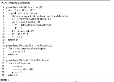
[image:7.486.55.441.63.340.2]24: returnγγγ Figure 1
The proposed ADF on-line learning algorithm. In the algorithm,ZZZis the training data set;q,c,α, andβare hyper-parameters;qis an integer representing window size;cis for initializing the learning rates; andαandβare the upper and lower bounds of a scalar, with 0< β < α <1.
With this setting, different features correspond to different adaptation factors based on feature frequency information. Our ADF algorithm is summarized in Figure 1.
The ADF training method is efficient because the only additional computation (compared with traditional SGD) is the derivation of the learning rates, which is simple and efficient. As we know, the regularization of SGD can perform efficiently via the opti-mization based on sparse features (Shalev-Shwartz, Singer, and Srebro 2007). Similarly, the derivation ofγγγt can also perform efficiently via the optimization based on sparse features. Note that although binary features are common in natural language processing tasks, the ADF algorithm is not limited to binary features and it can be applied to real-valued features.
3.2 Convergence Analysis
We want to show that the proposed ADF learning algorithm has good convergence properties. There are two steps in the convergence analysis. First, we show that the ADF update rule is a contraction mapping. Then, we show that the ADF training is asymptotically convergent, and with a fast convergence rate.
To simplify the discussion, our convergence analysis is based on the convex loss function of traditional classification or regression problems:
L(www)= n ∑
i=1
ℓ(xxxi,yi,www·fffi)− ||
wherefffiis the feature vector generated from the training sample (xxxi,yi).L(www) is a
func-tion inwww·fffi, such as 12(yi−www·fffi)2 for regression or log[1+exp(−yiwww·fffi)] for binary
classification.
To make convergence analysis of the proposed ADF training algorithm, we need to introduce several mathematical definitions. First, we introduce Lipschitz continuity:
Definition 1 (Lipschitz continuity)
A function F:X →Ris Lipschitz continuous with the degree of Dif|F(x)−F(y)| ≤ D|x−y| for∀x,y∈X. X can be multi-dimensional space, and|x−y| is the distance between the pointsxandy.
Based on the definition of Lipschitz continuity, we give the definition of the Lipschitz constant||F||Lipas follows:
Definition 2 (Lipschitz constant)
||F||Lip:=inf{D where |F(x)−F(y)| ≤D|x−y| for ∀x,y}
In other words, the Lipschitz constant||F||Lipis the lower bound of the continuity degree that makes the functionFLipschitz continuous.
Further, based on the definition of Lipschitz constant, we give the definition of contraction mapping as follows:
Definition 3 (Contraction mapping)
A functionF:X →X is a contraction mapping if its Lipschitz constant is smaller than 1:||F||Lip<1.
Then, we can show that the traditional SGD update is a contraction mapping.
Lemma 1 (SGD update rule is contraction mapping)
Letγbe a fixed low learning rate in SGD updating. Ifγ≤(||x2
i|| · ||∇yyy′′′ℓ(xxxi,yi,y′)||Lip)−1,
the SGD update rule is a contraction mapping in Euclidean space with Lipschitz con-tinuity degree 1−γ/σ2.
The proof can be extended from the related work on convergence analysis of parallel SGD training (Zinkevich et al. 2010). The stochastic training process is a one-following-one dynamic update process. In this dynamic process, if we use the same update ruleF, we havewwwt+1=F(wwwt) andwwwt+2=F(wwwt+1). It is only necessary to prove that the dynamic update is a contraction mapping restricted by this one-following-one dynamic process. That is, for the proposed ADF update rule, it is only necessary to prove it is adynamic contraction mapping. We formally define dynamic contraction mapping as follows.
Definition 4 (Dynamic contraction mapping)
Given a functionF:X →X, suppose the function is used in a dynamic one-following-one process: xt+1 =F(xt) and xt+2 =F(xt+1) for ∀xt∈X. Then, the function F is a
dynamic contraction mapping if∃D<1,|xt+2−xt+1| ≤D|xt+1−xt|for∀xt∈X.
that the ADF update rule with afixedlearning rate vector of different learning rates is a dynamic contraction mapping.
Theorem 1 (ADF update rule with fixed learning rates)
Letγγγbe a fixed learning rate vector with different learning rates. Letγmaxbe the
max-imum learning rate in the learning rate vectorγγγ:γmax:=sup{γi where γi∈γγγ}. Then
ifγmax≤(||x2i|| · ||∇yyy′′ℓ′ (xxxi,yi,y′)||Lip)−1, the ADF update rule is a dynamic contraction
mapping in Euclidean space with Lipschitz continuity degree 1−γmax/σ2. The proof is sketched in Section 5.
Further, we need to prove that the ADF update rule with a decaying learning rate vector is a dynamic contraction mapping, because the real ADF algorithm has a decaying learning rate vector. In the decaying case, the condition thatγmax≤(||x2i|| · ||∇yyy′′′ℓ(xxxi,yi,y′)||Lip)−1 can be easily achieved, becauseγγγ continues to decay with an
exponential decaying rate. Even if theγγγis initialized with high values of learning rates, after a number of training passes (denoted asT)γγγTis guaranteed to be small enough so
thatγmax:=sup{γi where γi∈γγγT}and γmax≤(||x2i|| · ||∇yyy′′′ℓ(xxxi,yi,y′)||Lip)−1. Without
losing generality, our convergence analysis starts from the passTand we takeγγγTasγγγ0 in the following analysis. Thus, we can show that the ADF update rule with a decaying learning rate vector is a dynamic contraction mapping:
Theorem 2 (ADF update rule with decaying learning rates)
Let γγγt be a learning rate vector in the ADF learning algorithm, which is decaying
over the time t and with different decaying rates based on feature frequency infor-mation. Let γγγt start from a low enough learning rate vector γγγ0 such that γmax≤
(||x2
i|| · ||∇yyy′′′ℓ(xxxi,yi,y′)||Lip)−1, whereγmaxis the maximum element inγγγ0. Then, the ADF update rule with decaying learning rate vector is a dynamic contraction mapping in Euclidean space with Lipschitz continuity degree 1−γmax/σ2.
The proof is sketched in Section 5.
Based on the connections between ADF training and contraction mapping, we demonstrate the convergence properties of the ADF training method. First, we prove the convergence of the ADF training.
Theorem 3 (ADF convergence)
ADF training is asymptotically convergent. The proof is sketched in Section 5.
Further, we analyze the convergence rate of the ADF training. When we have the lowest learning rateγγγt+1=βγγγt, the expectation of the obtainedwwwtis as follows (Murata
1998; Hsu et al. 2009):
E(wwwt)=www∗+ t ∏
m=1
(III−γγγ0βmHHH(www∗))(www0−www∗)
wherewww∗ is the optimal weight vector, andHHHis the Hessian matrix of the objective function. The rate of convergence is governed by the largest eigenvalue of the function C
Theorem 4 (ADF convergence rate)
Assumeϕis the largest eigenvalue of the functionCCCt= ∏t
m=1(III−γγγ0βmHHH(www∗)). For the proposed ADF training, its convergence rate is bounded byϕ, and we have
ϕ≤exp{γγγ0λβ
β−1}
whereλis the minimum eigenvalue ofHHH(www∗). The proof is sketched in Section 5.
The convergence analysis demonstrates that the proposed method with feature-frequency-adaptive learning rates is convergent and the bound of convergence rate is analyzed. It demonstrates that increasing the values ofγγγ0 and β leads to a lower bound of the convergence rate. Because the bound of the convergence rate is just an up-bound rather than the actual convergence rate, we still need to conduct automatic tuning of the hyper-parameters, includingγγγ0 and β, for optimal convergence rate in practice. The ADF training method has a fast convergence rate because the feature-frequency-adaptive schema can avoid the fluctuations on updating the weights of high frequency features, and it can avoid the insufficient training on updating the weights of low frequency features. In the following sections, we perform experiments to confirm the fast convergence rate of the proposed method.
4. Evaluation
Our main focus is on training heavily structured classification models. We evaluate the proposal on three NLP structured classification tasks: biomedical named entity recogni-tion (Bio-NER), Chinese word segmentarecogni-tion, and noun phrase (NP) chunking. For the structured classification tasks, the ADF training is based on the CRF model (Lafferty, McCallum, and Pereira 2001). Further, to demonstrate that the proposed method is not limited to structured classification tasks, we also perform experiments on a structured binary classification task: sentiment-based text classification. For the non-structured classification task, the ADF training is based on the maximum entropy model (Berger, Della Pietra, and Della Pietra 1996; Ratnaparkhi 1996).
4.1 Biomedical Named Entity Recognition (Structured Classification)
The biomedical named entity recognition (Bio-NER) task is from the BIONLP-2004 shared task. The task is to recognize five kinds of biomedical named entities, including DNA, RNA,protein, cell line, and cell type, on the MEDLINE biomedical text mining corpus (Kim et al. 2004). A typical approach to this problem is to cast it as a sequential labeling task with theBIOencoding.
This data set consists of 20,546 training samples (from 2,000 MEDLINE article abstracts, with 472,006 word tokens) and 4,260 test samples. The properties of the data are summarized in Table 1. State-of-the-art systems for this task include Settles (2004), Finkel et al. (2004), Okanohara et al. (2006), Hsu et al. (2009), Sun, Matsuzaki, et al. (2009), and Tsuruoka, Tsujii, and Ananiadou (2009).
Table 1
Summary of the Bio-NER data set.
#Abstracts #Sentences #Words
Train 2,000 20,546 (10/abs) 472,006 (23/sen)
Test 404 4,260 (11/abs) 96,780 (23/sen)
Table 2
Feature templates used for the Bio-NER task.wiis the current word token on positioni.tiis the
POS tag on positioni.oiis the orthography mode on positioni.yiis the classification label on
positioni.yi−1yirepresents label transition.A× Brepresents a Cartesian product between
two sets.
Word Token–based Features:
{wi−2,wi−1,wi,wi+1,wi+2,wi−1wi,wiwi+1} ×{yi, yi−1yi}
Part-of-Speech (POS)–based Features:
{ti−2,ti−1,ti,ti+1,ti+2,ti−2ti−1,ti−1ti,titi+1,ti+1ti+2,ti−2ti−1ti,ti−1titi+1,titi+1ti+2} ×{yi, yi−1yi}
Orthography Pattern–based Features:
{oi−2,oi−1,oi,oi+1,oi+2,oi−2oi−1,oi−1oi,oioi+1,oi+1oi+2} ×{yi, yi−1yi}
information of the observation sequence (i.e.,xxx). The major reason for this simple real-ization of edge features in traditional CRF implementation is to reduce the dimension of features. To improve the model accuracy, we utilizerich edge featuresfollowing Sun, Wang, and Li (2012), in which local observation information ofxxxis combined in edge features just like the implementation of node features. A detailed introduction to rich edge features can be found in Sun, Wang, and Li (2012). Using the feature templates, we extract a high dimensional feature set, which contains 5.3×10⁷ features in total. Following prior studies, the evaluation metric for this task is the balanced F-score defined as 2PR/(P+R), wherePis precision andRis recall.
4.2 Chinese Word Segmentation (Structured Classification)
Chinese word segmentation aims to automatically segment character sequences into word sequences. Chinese word segmentation is important because it is the first step for most Chinese language information processing systems. Our experiments are based on the Microsoft Research data provided by The Second International Chinese Word Segmentation Bakeoff. In this data set, there are 8.8×10⁴ word-types, 2.4×10⁶ word-tokens, 5×10³character-types, and 4.1×10⁶character-tokens. State-of-the-art systems for this task include Tseng et al. (2005), Zhang, Kikui, and Sumita (2006), Zhang and Clark (2007), Gao et al. (2007), Sun, Zhang, et al. (2009), Sun (2010), Zhao et al. (2010), and Zhao and Kit (2011).
The feature engineering follows previous work on word segmentation (Sun, Wang, and Li 2012). Rich edge features are used. For the classification labelyi and the label
transitionyi−1yion positioni, we use the feature templates as follows (Sun, Wang, and
Li 2012):
r
Character bigrams located at positionsi−2,i−1,iandi+1.r
Whetherxjandxj+1are identical, forj=i−2, . . ., i+1.r
Whetherxjandxj+2are identical, forj=i−3, . . ., i+1.r
The character sequencexj,iif it matches a wordw∈U, with the constraint i−6<j<i. The itemxj,irepresents the character sequencexj. . .xi. Urepresents the unigram-dictionary collected from the training data.r
The character sequencexi,kif it matches a wordw∈U, with the constrainti<k<i+6.
r
The word bigram candidate [xj,i−1,xi,k] if it hits a word bigram [wi, wj]∈B, and satisfies the aforementioned constraints onjandk. Brepresents the word bigram dictionary collected from the training data.r
The word bigram candidate [xj,i, xi+1,k] if it hits a word bigram[wi, wj]∈B, and satisfies the aforementioned constraints onjandk.
All feature templates are instantiated with values that occurred in training samples. The extracted feature set is large, and there are 2.4×10⁷features in total. Our evaluation is based on a closed test, and we do not use extra resources. Following prior studies, the evaluation metric for this task is the balanced F-score.
4.3 Phrase Chunking (Structured Classification)
In the phrase chunking task, the non-recursive cores of noun phrases, called base NPs, are identified. The phrase chunking data is extracted from the data of the CoNLL-2000 shallow-parsing shared task (Sang and Buchholz 2000). The training set consists of 8,936 sentences, and the test set consists of 2,012 sentences. We use the feature templates based on wordn-grams and part-of-speechn-grams, and feature templates are shown in Table 3. Rich edge features are used. Using the feature templates, we extract 4.8×10⁵ features in total. State-of-the-art systems for this task include Kudo and Matsumoto (2001), Collins (2002), McDonald, Crammer, and Pereira (2005), Vishwanathan et al. (2006), Sun et al. (2008), and Tsuruoka, Tsujii, and Ananiadou (2009). Following prior studies, the evaluation metric for this task is the balanced F-score.
4.4 Sentiment Classification (Non-Structured Classification)
To demonstrate that the proposed method is not limited to structured classification, we select a well-known sentiment classification task for evaluating the proposed method on non-structured classification.
Table 3
Feature templates used for the phrase chunking task.wi,ti, andyiare defined as before.
Word-Token–based Features:
{wi−2,wi−1,wi,wi+1,wi+2,wi−1wi,wiwi+1} ×{yi, yi−1yi}
Part-of-Speech (POS)–based Features:
Generally, sentiment classification classifies user review text as a positive or neg-ative opinion. This task (Blitzer, Dredze, and Pereira 2007) consists of four subtasks based on user reviews from Amazon.com. Each subtask is a binary sentiment clas-sification task based on a specific topic. We use the maximum entropy model for classification. We use the same lexical features as those used in Blitzer, Dredze, and Pereira (2007), and the total number of features is 9.4×10⁵. Following prior work, the evaluation metric is binary classification accuracy.
4.5 Experimental Setting
As for training, we perform gradient descent with the proposed ADF training method. To compare with existing literature, we choose four popular training methods, a rep-resentative batch training method, and three reprep-resentative on-line training methods. The batch training method is the limited-memory BFGS (LBFGS) method (Nocedal and Wright 1999), which is considered to be one of the best optimizers for log-linear models like CRFs. The on-line training methods include the SGD training method, which we introduced in Section 2.2, the structured perceptron (Perc) training method (Freund and Schapire 1999; Collins 2002), and the averaged perceptron (Avg-Perc) training method (Collins 2002). The structured perceptron method and averaged perceptron method are non-probabilistic training methods that have very fast training speed due to the avoidance of the computation on gradients (Sun, Matsuzaki, and Li 2013). All training methods, including ADF, SGD, Perc, Avg-Perc, and LBFGS, use the same set of features.
We also compared the ADF method with the CW method (Dredze, Crammer, and Pereira 2008) and the AROW method (Crammer, Kulesza, and Dredze 2009). The CW and AROW methods are implemented based on the Confidence Weighted Learning Library.2 Because the current implementation of the CW and AROW methods do not utilize rich edge features, we removed the rich edge features in our systems to make more fair comparisons. That is, we removed rich edge features in the CRF-ADF setting, and this simplified method is denoted as ADF-noRich. The second-order stochastic gradient descent training methods, including the SMD method (Vishwanathan et al. 2006) and the PSA method (Hsu et al. 2009), are not considered in our experiments because we find those methods are quite slow when running on our data sets with high dimensional features.
We find that the settings ofq,α, andβin the ADF training method are not sensitive among specific tasks and can be generally set. We simply setq=n/10 (nis the number of training samples). It means that feature frequency information is updated 10 times per iteration. Via cross-validation only on the training data of different tasks, we find that the following setting is sufficient to produce adequate performance for most of the real-world natural language processing tasks:α around 0.995 andβ around 0.6. This indicates that the feature frequency information has similar characteristics across many different natural language processing tasks.
Thus, we simply use the following setting for all tasks: q=n/10, α=0.995, and
β=0.6. This leavesc(the initial value of the learning rates) as the only hyper-parameter that requires careful tuning. We perform automatic tuning forcbased on the training data via 4-fold cross-validation, testing withc=0.005, 0.01, 0.05, 0.1, respectively, and the optimalcis chosen based on the best accuracy of cross-validation. Via this automatic
tuning, we find it is proper to set c=0.005, 0.1, 0.05, 0.005, for the Bio-NER, word segmentation, phrase chunking, and sentiment classification tasks, respectively.
To reduce overfitting, we use an L2 Gaussian weight prior (Chen and Rosenfeld 1999) for the ADF, LBFGS, and SGD training methods. We vary the σ with different values (e.g., 1.0, 2.0, and 5.0) for 4-fold cross validation on the training data of different tasks, and finally setσ=5.0 for all training methods in the Bio-NER task;σ=5.0 for all training methods in the word segmentation task; σ=5.0, 1.0, 1.0 for ADF, SGD, and LBFGS in the phrase chunking task; and σ=1.0 for all training methods in the sentiment classification task. Experiments are performed on a computer with an Intel(R) Xeon(R) 2.0-GHz CPU.
4.6 Structured Classification Results
4.6.1 Comparisons Based on Empirical Convergence.First, we check the experimental re-sults of different methods on their empirical convergence state. Because the perceptron training method (Perc) does not achieve empirical convergence even with a very large number of training passes, we simply report its results based on a large enough number of training passes (e.g., 200 passes). Experimental results are shown in Table 4.
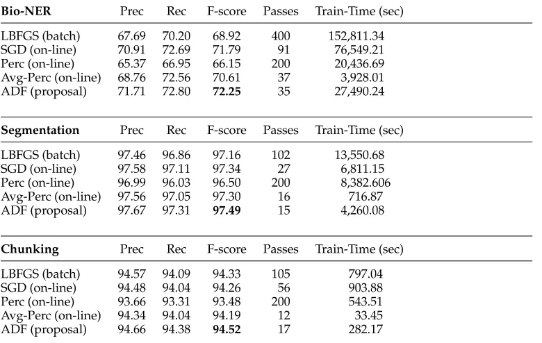
[image:14.486.49.439.417.664.2]As we can see, the proposed ADF method is more accurate than other training methods, either the on-line ones or the batch one. It is a bit surprising that the ADF method performs even more accurately than the batch training method (LBFGS). We notice that some previous work also found that on-line training methods could have
Table 4
Results for the Bio-NER, word segmentation, and phrase chunking tasks. The results and the number of passes are decided based on empirical convergence (with score deviation of adjacent five passes less than 0.01). For the non-convergent case, we simply report the results based on a large enough number of training passes. As we can see, the ADF method achieves the best accuracy with the fastest convergence speed.
Bio-NER Prec Rec F-score Passes Train-Time (sec)
LBFGS (batch) 67.69 70.20 68.92 400 152,811.34
SGD (on-line) 70.91 72.69 71.79 91 76,549.21
Perc (on-line) 65.37 66.95 66.15 200 20,436.69
Avg-Perc (on-line) 68.76 72.56 70.61 37 3,928.01
ADF (proposal) 71.71 72.80 72.25 35 27,490.24
Segmentation Prec Rec F-score Passes Train-Time (sec)
LBFGS (batch) 97.46 96.86 97.16 102 13,550.68
SGD (on-line) 97.58 97.11 97.34 27 6,811.15
Perc (on-line) 96.99 96.03 96.50 200 8,382.606
Avg-Perc (on-line) 97.56 97.05 97.30 16 716.87
ADF (proposal) 97.67 97.31 97.49 15 4,260.08
Chunking Prec Rec F-score Passes Train-Time (sec)
LBFGS (batch) 94.57 94.09 94.33 105 797.04
SGD (on-line) 94.48 94.04 94.26 56 903.88
Perc (on-line) 93.66 93.31 93.48 200 543.51
Avg-Perc (on-line) 94.34 94.04 94.19 12 33.45
better performance than batch training methods such as LBFGS (Tsuruoka, Tsujii, and Ananiadou 2009; Schaul, Zhang, and LeCun 2012). The ADF training method can achieve better results probably because the feature-frequency–adaptive training schema can produce more balanced training of features with diversified frequencies. Traditional SGD training may over-train high frequency features and at the same time may have insufficient training of low frequency features. The ADF training method can avoid such problems. It will be interesting to perform further analysis in future work.
We also performed significance tests based on t-tests with a significance level of 0.05. Significance tests demonstrate that the ADF method is significantly more accurate than the existing training methods in most of the comparisons, whether on-line or batch. For the Bio-NER task, the differences between ADF and LBFGS, SGD, Perc, and Avg-Perc are significant. For the word segmentation task, the differences between ADF and LBFGS, SGD, Perc, and Avg-Perc are significant. For the phrase chunking task, the differences between ADF and Perc and Avg-Perc are significant; the differences between ADF and LBFGS and SGD are non-significant.
Moreover, as we can see, the proposed method achieves a convergence state with the least number of training passes, and with the least wall-clock time. In general, the ADF method is about one order of magnitude faster than the LBFGS batch training method and several times faster than the existing on-line training methods.
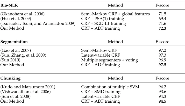
4.6.2 Comparisons with State-of-the-Art Systems.The three tasks are well-known bench-mark tasks with standard data sets. There is a large amount of published research on those three tasks. We compare the proposed method with the state-of-the-art systems. The comparisons are shown in Table 5.
[image:15.486.53.436.444.664.2]As we can see, our system is competitive with the best systems for the Bio-NER, word segmentation, and NP-chunking tasks. Many of the state-of-the-art systems use extra resources (e.g., linguistic knowledge) or complicated systems (e.g., voting over
Table 5
Comparing our results with some representative state-of-the-art systems.
Bio-NER Method F-score
(Okanohara et al. 2006) Semi-Markov CRF + global features 71.5
(Hsu et al. 2009) CRF + PSA(1) training 69.4
(Tsuruoka, Tsujii, and Ananiadou 2009) CRF + SGD-L1 training 71.6
Our Method CRF + ADF training 72.3
Segmentation Method F-score
(Gao et al. 2007) Semi-Markov CRF 97.2
(Sun, Zhang, et al. 2009) Latent-variable CRF 97.3
(Sun 2010) Multiple segmenters + voting 96.9
Our Method CRF + ADF training 97.5
Chunking Method F-score
(Kudo and Matsumoto 2001) Combination of multiple SVM 94.2
(Vishwanathan et al. 2006) CRF + SMD training 93.6
(Sun et al. 2008) Latent-variable CRF 94.3
multiple models). Thus, it is impressive that our single model–based system without extra resources achieves good performance. This indicates that the proposed ADF training method can train model parameters with good generality on the test data.
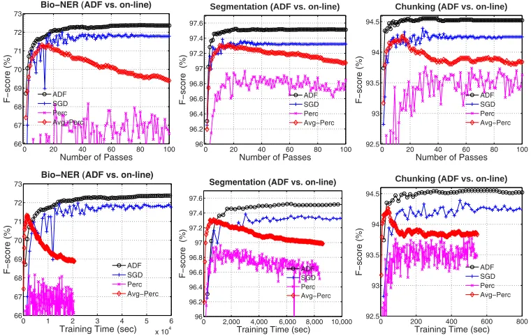
4.6.3 Training Curves.To study the detailed training process and convergence speed, we show the training curves in Figures 2–4. Figure 2 focuses on the comparisons between the ADF method and the existing on-line training methods. As we can see, the ADF method converges faster than other on-line training methods in terms of both training passes and wall-clock time. The ADF method has roughly the same training speed per pass compared with traditional SGD training.
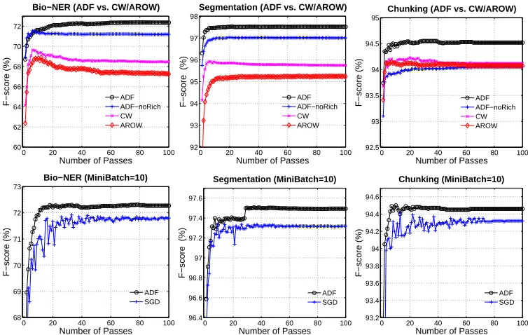
[image:16.486.49.429.362.603.2]Figure 3 (Top Row) focuses on comparing the ADF method with the CW method (Dredze, Crammer, and Pereira 2008) and the AROW method (Crammer, Kulesza, and Dredze 2009). Comparisons are based on similar features. As discussed before, the ADF-noRich method is a simplified system, with rich edge features removed from the CRF-ADF system. As we can see, the proposed CRF-ADF method, whether with or without rich edge features, outperforms the CW and AROW methods. Figure 3 (Bottom Row) focuses on the comparisons with different mini-batch(the training samples in each stochastic update) sizes. Representative results with a mini-batch size of 10 are shown. In general, we find larger mini-batch sizes will slow down the convergence speed. Results demon-strate that, compared with the SGD training method, the ADF training method is less sensitive to mini-batch sizes.
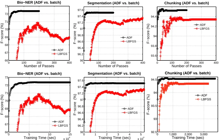
Figure 4 focuses on the comparisons between the ADF method and the batch training method LBFGS. As we can see, the ADF method converges at least one order
0 20 40 60 80 100 66 67 68 69 70 71 72 73
Number of Passes
)
ADF SGD Perc
0 20 40 60 80 100 96 96.2 96.4 96.6 96.8 97 97.2 97.4 97.6
Segmentation (ADF vs. on-line)
Number of Passes
)
ADF SGD Perc
0 20 40 60 80 100
92.5 93 93.5 94 94.5
Chunking (ADF vs. on-line)
Number of Passes
)
ADF SGD Perc
0 1 2 3 4 5 6
x 104 66 67 68 69 70 71 72 73
Training Time (sec)
)
ADF SGD Perc
0 2,000 4,000 6,000 8,000 10,000 96 96.2 96.4 96.6 96.8 97 97.2 97.4 97.6
Segmentation (ADF vs. on-line)
Training Time (sec)
)
ADF SGD Perc
0 200 400 600 800
92.5 93 93.5 94 94.5
Chunking (ADF vs. on-line)
Training Time (sec)
)
ADF SGD Perc
Figure 2
0 20 40 60 80 100 60 62 64 66 68 70 72
Bio−NER (ADF vs. CW/AROW)
Number of Passes
F−score (%) ADFADF−noRich
CW AROW
0 20 40 60 80 100 92 93 94 95 96 97 98
Segmentation (ADF vs. CW/AROW)
Number of Passes
F−score (%) ADFADF−noRich
CW AROW
0 20 40 60 80 100 92.5 93 93.5 94 94.5 95
Chunking (ADF vs. CW/AROW)
Number of Passes
F−score (%) ADFADF−noRich
CW AROW
0 20 40 60 80 100 68 69 70 71 72 73 Bio−NER (MiniBatch=10)
Number of Passes
F−score (%)
ADF SGD
0 20 40 60 80 100 96.4 96.6 96.8 97 97.2 97.4 97.6 Segmentation (MiniBatch=10)
Number of Passes
F−score (%)
ADF SGD
0 20 40 60 80 100 93.2 93.4 93.6 93.8 94 94.2 94.4 94.6 Chunking (MiniBatch=10)
Number of Passes
F−score (%)
[image:17.486.54.431.64.303.2]ADF SGD
Figure 3
(Top Row) Comparing ADF and ADF-noRich with CW and AROW methods. As we can see, both the ADF and ADF-noRich methods work better than the CW and AROW methods. (Bottom Row) Comparing different methods with mini-batch = 10 in the stochastic learning setting.
magnitude faster than the LBFGS training in terms of both training passes and wall-clock time. For the LBFGS training, we need to determine the LBFGS memory parameter m, which controls the number of prior gradients used to approximate the Hessian information. A larger value of m will potentially lead to more accurate estimation of the Hessian information, but at the same time will consume significantly more memory. Roughly, the LBFGS training consumesmtimes more memory than the ADF on-line training method. For most tasks, the default setting ofm=10 is reasonable. We setm=10 for the word segmentation and phrase chunking tasks, and m=6 for the Bio-NER task due to the shortage of memory form>6 cases in this task.
4.6.4 One-Pass Learning Results.Many real-world data sets can only observe the training data in one pass. For example, some Web-based on-line data streams can only appear once so that the model parameter learning should be finished in one-pass learning (see Zinkevich et al. 2010). Hence, it is important to test the performance in the one-pass learning scenario.
0 100 200 300 400 66 67 68 69 70 71 72 73
Bio−NER (ADF vs. batch)
Number of Passes
F−score (%)
ADF LBFGS
0 100 200 300 400 96 96.2 96.4 96.6 96.8 97 97.2 97.4 97.6
Segmentation (ADF vs. batch)
Number of Passes
F−score (%)
ADF LBFGS
0 100 200 300 400 93.6
93.8 94 94.2 94.4
Chunking (ADF vs. batch)
Number of Passes
F−score (%)
ADF LBFGS
0 5 10 15
x 104 66 67 68 69 70 71 72 73
Bio−NER (ADF vs. batch)
Training Time (sec)
F−score (%)
ADF LBFGS
0 1 2 3 4 5
x 104 96 96.2 96.4 96.6 96.8 97 97.2 97.4 97.6
Segmentation (ADF vs. batch)
Training Time (sec)
F−score (%)
ADF LBFGS
0 1,000 2,000 3,000
92.5 93 93.5 94 94.5
Chunking (ADF vs. batch)
Training Time (sec)
) ADF
[image:18.486.51.428.65.306.2]LBFGS
Figure 4
Comparisons between the ADF method and the batch training method LBFGS. (Top Row) Comparisons based on training passes. As we can see, the ADF method converges much faster than the LBFGS method, and with better accuracy on the convergence state. (Bottom Row) Comparisons based on wall-clock time.
consistently outperforms the baselines. This also reflects the fast convergence speed of the ADF training method.
4.7 Non-Structured Classification Results
[image:18.486.48.437.514.630.2]In previous experiments, we showed that the proposed method outperforms existing baselines on structured classification. Nevertheless, we want to show that the ADF method also has good performance on non-structured classification. In addition, this task is based on real-valued features instead of binary features.
Figure 5
Table 6
Results on sentiment classification (non-structured binary classification).
Accuracy Passes Train-Time (sec)
LBFGS (batch) 87.00 86 72.20
SGD (on-line) 87.13 44 55.88
Perc (on-line) 84.55 25 5.82
Avg-Perc (on-line) 85.04 46 12.22
ADF (proposal) 87.89 30 57.12
Experimental results of different training methods on the convergence state are shown in Table 6. As we can see, the proposed method outperforms all of the on-line and batch baselines in terms of binary classification accuracy. Here again we observe that the ADF and SGD methods outperform the LBFGS baseline.
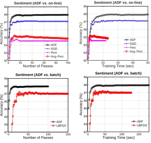
The training curves are shown in Figure 6. As we can see, the ADF method con-verges quickly. Because this data set is relatively small and the feature dimension is much smaller than previous tasks, we find the baseline training methods also have fast convergence speed. The comparisons on one-pass learning are shown in Fig-ure 7. Just as for the experiments for structFig-ured classification tasks, the ADF method
0 20 40 60 80 100 82
83 84 85 86 87 88 89
Sentiment (ADF vs. on-line)
Number of Passes
Accuracy (%
)
ADF SGD Perc
0 20 40 60 80
82 83 84 85 86 87 88 89
Sentiment (ADF vs. on-line)
Training Time (sec)
Accuracy (%
)
ADF SGD Perc
0 50 100 150
82 83 84 85 86 87 88 89
Sentiment (ADF vs. batch)
Number of Passes
Accuracy (%)
ADF LBFGS
0 50 100 150 82
83 84 85 86 87 88 89
Sentiment (ADF vs. batch)
Training Time (sec)
Accuracy (%)
[image:19.486.54.317.339.588.2]ADF LBFGS
Figure 6
Figure 7
One-pass learning results on sentiment classification.
outperforms the baseline methods on one-pass learning, with more than 12.7% error rate reduction.
5. Proofs
This section gives proofs of Theorems 1–4.
Proof of Theorem 1Following Equation (5), the ADF update rule isF(wwwt) :=wwwt+1= w
w
wt+γγγ···gggt. For∀wwwt∈X,
|F(wwwt+1)−F(wwwt)| =|F(wwwt+1)−wwwt+1|
=|wwwt+1+γγγ···gggt+1−wwwt+1|
=|γγγ···gggt+1|
=[(a1b1)2+(a2b2)2+· · ·+(afbf)2]1/2
≤[(γmaxb1)2+(γmaxb2)2+· · ·+(γmaxbf)2]1/2
=|γmaxgggt+1|
=|FSGD(wwwt+1)−FSGD(wwwt)|
(6)
whereai andbi are theith elements of the vectorγγγandgggt+1, respectively.FSGD is the
SGD update rule with the fixed learning rateγmaxsuch thatγmax:=sup{γi where γi∈ γ
γ
γ}. In other words, for the SGD update ruleFSGD, the fixed learning rateγmaxis derived
from the ADF update rule. According to Lemma 1, the SGD update rule FSGD is a
contraction mapping in Euclidean space with Lipschitz continuity degree 1−γmax/σ2,
given the condition thatγmax≤(||x2i|| · ||∇yyy′′′ℓ(xxxi,yi,y′)||Lip)−1. Hence, it goes to
|FSGD(wwwt+1)−FSGD(wwwt)| ≤(1−γmax/σ2)|wwwt+1−wwwt| (7)
Combining Equations (6) and (7), it goes to
|F(wwwt+1)−F(wwwt)| ≤(1−γmax/σ2)|wwwt+1−wwwt|
Thus, according to the definition of dynamic contraction mapping, the ADF update rule is a dynamic contraction mapping in Euclidean space with Lipschitz continuity degree
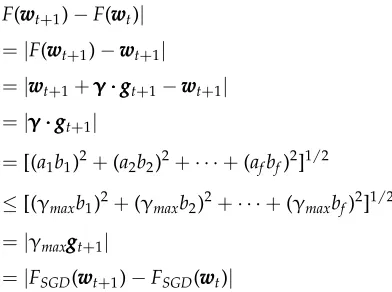
Proof of Theorem 2As presented in Equation (5), the ADF update rule isF(wwwt) :=
w
wwt+1=wwwt+γγγt···gggt. For∀wwwt∈X,
|F(wwwt+1)−F(wwwt)| =|γγγt+1···gggt+1|
=[(a1b1)2+(a2b2)2+· · ·+(afbf)2]1/2
≤[(γmaxb1)2+(γmaxb2)2+· · ·+(γmaxbf)2]1/2
=|FSGD(wwwt+1)−FSGD(wwwt)|
(8)
where ai is the ith element of the vector γγγt+1. bi and FSGD are the same as before.
Similar to the analysis of Theorem 1, the third step of Equation (8) is valid becauseγmax
is the maximum learning rate at the beginning and all learning rates are decreasing whentis increasing. The proof can be easily derived following the same steps in the proof of Theorem 1. To avoid redundancy, we do not repeat the derivation. ⊓⊔
Proof of Theorem 3LetMbe theaccumulative changeof the ADF weight vectorwwwt:
Mt:= ∑
t′=1,2,...,t
|wwwt′+1−wwwt′|
To prove the convergence of the ADF, we need to prove the sequenceMtconverges as
t→ ∞. Following Theorem 2, we have the following formula for the ADF training:
|F(wwwt+1)−F(wwwt)| ≤(1−γmax/σ2)|wwwt+1−wwwt|
where γmax is the maximum learning rate at the beginning. Let d0:=|www2−www1| and q:=1−γmax/σ2, then we have:
Mt= ∑
t′=1,2,...,t
|wwwt′+1−wwwt′|
≤d0+d0q+d0q2+· · ·+d0qt−1
=d0(1−qt)/(1−q)
(9)
Whent→ ∞,d0(1−qt)/(1−q) goes tod0/(1−q) becauseq<1. Hence, we have:
Mt≤d0/(1−q)
Thus,Mt is upper-bounded. Because we know thatMtis a monotonically increasing
function whent→ ∞, it follows thatMtconverges when t→ ∞. This completes the
Proof of Theorem 4First, we have
eigen(CCCt)= t ∏
m=1
(1−γγγ0βmλ)
≤exp
{ −γγγ0λ
t ∑
m=1
βm
}
Then, we have
0≤
n ∏
j=1
(1−aj)≤ n ∏
j=1
e−aj=e−
∑n
j=1aj
This is because 1−aj≤e−aj given 0≤aj<1. Finally, because ∑t
m=1βm → 1−ββ when
t→ ∞, we have
eigen(CCCt)≤exp {
−γγγ0λ
t ∑
m=1
βm
}
→exp
{ −γγγ0λβ
1−β }
This completes the proof. ⊓⊔
6. Conclusions
In this work we tried to simultaneously improve the training speed and model accuracy of natural language processing systems. We proposed the ADF on-line training method, based on the core idea that high frequency features should result in a learning rate that decays faster. We demonstrated that the ADF on-line training method is convergent and has good theoretical properties. Based on empirical experiments, we can state the following conclusions. First, the ADF method achieved the major target of this work: faster training speed and higher accuracy at the same time. Second, the ADF method was robust: It had good performance on several structured and non-structured classifi-cation tasks with very different characteristics. Third, the ADF method worked well on both binary features and real-valued features. Fourth, the ADF method outperformed existing methods in a one-pass learning setting. Finally, our method achieved state-of-the-art performance on several well-known benchmark tasks. To the best of our knowledge, our simple method achieved a much better F-score than the existing best reports on the biomedical named entity recognition task.
Acknowledgments
This work was supported by the National Natural Science Foundation of China (no. 61300063, no. 61370117), the Doctoral Fund of Ministry of Education of China (no. 20130001120004), a Hong Kong Polytechnic University internal grant (4-ZZD5), a Hong Kong RGC Project
(no. PolyU 5230/08E), the National High Technology Research and Development Program of China (863 Program,
References
Berger, Adam L., Vincent J. Della Pietra, and Stephen A. Della Pietra. 1996. A maximum entropy approach to natural language processing.Computational Linguistics, 22(1):39–71.
Blitzer, John, Mark Dredze, and Fernando Pereira. 2007. Biographies, Bollywood, boom-boxes and blenders: Domain adaptation for sentiment classification. InProceedings of the 45th Annual Meeting of the Association of Computational Linguistics, pages 440–447, Prague.
Bottou, L´eon. 1998. Online algorithms and stochastic approximations. In D. Saad, editor.Online Learning and Neural Networks. Cambridge University Press, pages 9–42.
Chen, Stanley F. and Ronald Rosenfeld. 1999. A Gaussian prior for smoothing maximum entropy models. Technical Report CMU-CS-99-108, Carnegie Mellon University.
Collins, Michael. 2002. Discriminative training methods for hidden Markov models: Theory and experiments with perceptron algorithms. InProceedings of EMNLP’02, pages 1–8, Philadelphia, PA. Crammer, Koby, Alex Kulesza, and Mark
Dredze. 2009. Adaptive regularization of weight vectors. InNIPS’09, pages 414–422, Vancouver.
Dredze, Mark, Koby Crammer, and Fernando Pereira. 2008. Confidence-weighted linear classification. In
Proceedings of ICML’08, pages 264–271, Helsinki.
Duchi, John, Elad Hazan, and Yoram Singer. 2010. Adaptive subgradient methods for online learning and stochastic optimization.Journal of Machine Learning Research, 12:2,121–2,159.
Finkel, Jenny, Shipra Dingare, Huy Nguyen, Malvina Nissim, Christopher Manning, and Gail Sinclair. 2004. Exploiting context for biomedical entity recognition: From syntax to the Web. InProceedings of BioNLP’04, pages 91–94, Geneva. Freund, Yoav and Robert Schapire. 1999.
Large margin classification using the perceptron algorithm.Machine Learning, 37(3):277–296.
Gao, Jianfeng, Galen Andrew, Mark Johnson, and Kristina Toutanova. 2007. A comparative study of parameter estimation methods for statistical natural language processing. In
Proceedings of the 45th Annual Meeting of the Association of Computational Linguistics (ACL’07), pages 824–831, Prague.
Hsu, Chun-Nan, Han-Shen Huang, Yu-Ming Chang, and Yuh-Jye Lee. 2009. Periodic step-size adaptation in second-order gradient descent for single-pass on-line structured learning.Machine Learning, 77(2-3):195–224.
Jacobs, Robert A. 1988. Increased rates of convergence through learning rate adaptation.Neural Networks, 1(4):295–307. Kim, Jin-Dong, Tomoko Ohta, Yoshimasa
Tsuruoka, and Yuka Tateisi. 2004. Introduction to the bio-entity recognition task at JNLPBA. InProceedings of
BioNLP’04, pages 70–75, Geneva. Kudo, Taku and Yuji Matsumoto. 2001.
Chunking with support vector machines. InProceedings of NAACL’01, pages 1–8, Pittsburgh, PA.
Lafferty, John, Andrew McCallum, and Fernando Pereira. 2001. Conditional random fields: Probabilistic models for segmenting and labeling sequence data. InICML’01, pages 282–289, Williamstown, MA.
McDonald, Ryan, Koby Crammer, and Fernando Pereira. 2005. Flexible text segmentation with structured multilabel classification. InProceedings of HLT/ EMNLP’05, pages 987–994, Vancouver. McMahan, H. Brendan and Matthew J.
Streeter. 2010. Adaptive bound optimization for online convex
optimization. InProceedings of COLT’10, pages 244–256, Haifa.
Murata, Noboru. 1998. A statistical study of on-line learning. In D. Saad, editor.
Online Learning in Neural Networks. Cambridge University Press, pages 63–92. Nocedal, Jorge and Stephen J. Wright.
1999.Numerical optimization. Springer. Okanohara, Daisuke, Yusuke Miyao,
Yoshimasa Tsuruoka, and Jun’ichi Tsujii. 2006. Improving the scalability of semi-Markov conditional random fields for named entity recognition. InProceedings of COLING-ACL’06, pages 465–472, Sydney.
Ratnaparkhi, Adwait. 1996. A maximum entropy model for part-of-speech tagging. InProceedings of the Conference on Empirical Methods in Natural Language Processing 1996, pages 133–142, Pennsylvania. Sang, Erik Tjong Kim and Sabine Buchholz.
2000. Introduction to the CoNLL-2000 shared task: Chunking. InProceedings of CoNLL’00, pages 127–132, Lisbon. Schaul, Tom, Sixin Zhang, and Yann LeCun.
Settles, Burr. 2004. Biomedical named entity recognition using conditional random fields and rich feature sets. InProceedings of BioNLP’04, pages 104–107, Geneva. Shalev-Shwartz, Shai, Yoram Singer, and
Nathan Srebro. 2007. Pegasos: Primal estimated sub-gradient solver for SVM. InProceedings of ICML’07, pages 807–814, Corvallis, OR.
Sperduti, Alessandro and Antonina Starita. 1993. Speed up learning and network optimization with extended back
propagation.Neural Networks, 6(3):365–383. Sun, Weiwei. 2010. Word-based and
character-based word segmentation models: Comparison and combination. InCOLING’10 (Posters), pages 1,211–1,219, Beijing.
Sun, Xu, Takuya Matsuzaki, and Wenjie Li. 2013. Latent structured perceptrons for large-scale learning with hidden information.IEEE Transactions on Knowledge and Data Engineering, 25(9):2,063–2,075.
Sun, Xu, Takuya Matsuzaki, Daisuke Okanohara, and Jun’ichi Tsujii. 2009. Latent variable perceptron algorithm for structured classification. InProceedings of the 21st International Joint Conference on Artificial Intelligence (IJCAI 2009), pages 1,236–1,242, Pasadena, CA. Sun, Xu, Louis-Philippe Morency, Daisuke
Okanohara, and Jun’ichi Tsujii. 2008. Modeling latent-dynamic in shallow parsing: A latent conditional model with improved inference. InProceedings of COLING’08, pages 841–848, Manchester. Sun, Xu, Houfeng Wang, and Wenjie Li. 2012.
Fast online training with frequency-adaptive learning rates for Chinese word segmentation and new word detection. InProceedings of ACL’12, pages 253–262, Jeju Island.
Sun, Xu, Yaozhong Zhang, Takuya Matsuzaki, Yoshimasa Tsuruoka, and Jun’ichi Tsujii. 2009. A discriminative latent variable Chinese segmenter with hybrid word/character information. InProceedings of NAACL-HLT’09, pages 56–64, Boulder, CO. Sun, Xu, Yao Zhong Zhang, Takuya
Matsuzaki, Yoshimasa Tsuruoka, and Jun’ichi Tsujii. 2013. Probabilistic Chinese
word segmentation with non-local information and stochastic training.
Information Processing & Management, 49(3):626–636.
Tseng, Huihsin, Pichuan Chang, Galen Andrew, Daniel Jurafsky, and Christopher Manning. 2005. A conditional random field word segmenter for SIGHAN bakeoff 2005. InProceedings of the Fourth SIGHAN Workshop, pages 168–171, Jeju Island. Tsuruoka, Yoshimasa, Jun’ichi Tsujii, and
Sophia Ananiadou. 2009. Stochastic gradient descent training for
l1-regularized log-linear models with cumulative penalty. InProceedings of ACL’09, pages 477–485, Suntec. Vishwanathan, S. V. N., Nicol N.
Schraudolph, Mark W. Schmidt, and Kevin P. Murphy. 2006. Accelerated training of conditional random fields with stochastic meta-descent. InProceedings of ICML’06, pages 969–976, Pittsburgh, PA.
Zhang, Ruiqiang, Genichiro Kikui, and Eiichiro Sumita. 2006. Subword-based tagging by conditional random fields for Chinese word segmentation. InProceedings of the Human Language Technology
Conference of the NAACL, Companion Volume: Short Papers, pages 193–196, New York City.
Zhang, Yue and Stephen Clark. 2007. Chinese segmentation with a word-based perceptron algorithm. InProceedings of the 45th Annual Meeting of the Association of Computational Linguistics, pages 840–847, Prague.
Zhao, Hai, Changning Huang, Mu Li, and Bao-Liang Lu. 2010. A unified character-based tagging framework for Chinese word segmentation.ACM Transactions on Asian Language Information Processing, 9(2): Article 5.
Zhao, Hai and Chunyu Kit. 2011. Integrating unsupervised and supervised word segmentation: The role of goodness measures.Information Sciences, 181(1):163–183.