Uncertainty through Polynomial Chaos
in the EEG Problem
Rob H. De Staelen
Abstract—A sensitivity and correlation analysis of EEG sensors influenced by uncertain conductivity is conducted. We assume a three layer spherical head model with different and random layer conductivities. This randomness is modeled by Polynomial Chaos (PC). On average, we observe the least influenced electrodes along the great longitudinal fissure. Also, sensors located closer to a dipole source, are of greater influence to a change in conductivity – this is in agreement with previous research. The highly influenced sensors were on average located temporal. This was also the case in the correlation analysis, which was made possible by our approach with PC. Sensors in the temporal parts of the brain are highly correlated. Whereas the sensors in the occipital and lower frontal region, though they are close together, are not so highly correlated as in the temporal regions.
Index Terms—Polynomial Chaos, Electroencephalography, Uncertain conductivity, Sensitivity analysis, Correlation anal-ysis.
I. INTRODUCTION
E
LECTROENCEPHALOGRAPHY (EEG) is one of themost influential tools in the diagnosis of epilepsy and seizures, as it provides a record of ongoing electrical activity in the brain [1], [2]. The electrodes, connected to the EEG machine, measure signals produced by electrical discharge of neurons in the brain. The quasi-static approximation of the Maxwell equations is justified by the very low frequencies (typically <100 Hz) involved. The total electric current Jcan be partitioned [3] into two flows: a primary (driving) current Jp related to neural sources, and an ohmic volume
(passive) currentJvthat results from the effect of the electric
field in the volume:J=Jp+Jv=Jp+σE=Jp
−σ∇V, where V is the electric potential. Since the total current is divergence free and no current flows outside the head, we obtain
∇·(σ(r)∇V(r)) =∇·Jp(r), in H (1)
ν·σ(r)∇V(r) = 0, on ∂H (2)
whereH is the head,σthe conductivity andν the outward unit normal on∂H.
A. Model assumptions
Usually, the head is assumed to be made up of disjoint lay-ered regions (the scalp, skull, cerebrospinal fluid, grey matter and white matter, etc.) in each of which the conductivity is constant. We will use a spherical head model with three
layers: the inner sphere (radius.87) represents the brain, the intermediate layer (radius .92) represents the skull an the outer sphere (radius 1) corresponds to the scalp, see Fig.
Manuscript received November 19, 2010; revised January 17, 2011. R. De Staelen is with the Research Group of Numerical Analysis and Mathematical Modeling at the Department of Mathematical Analysis, Ghent University, B-9000 Ghent, Belgium (e-mail: Rob.DeStaelen@UGent.be).
1(b). The outer and inner layer are assumed to have similar electrical properties, meaning that σscalp =σbrain. Although we only consider a fixed (spherical) geometry, more realistic models exist and the effect of choice has been studied [4].
A widely used approximation of the neural activity of patients suffering from epilepsy [5] is the representation of the primary current as an electric dipole with dipole moment
dlocated atrd inside the cortex;Jp(r) =dδ(r−rd) with
r the position in the head measured from the center of the
concentric spheres andδ the Dirac measure. It is clear that
the sensitivity and correlation of the electrodes is key for a full understanding of EEG measurements.
B. Aim and novelty
The conductivity is in fact not constant in each layer and determining the conductivity values in the human head has been subject of research since many years [6]. Instead of working with the two different conductivitiesσskullandσbrain, we consider the conductivity ratio X =σscull/σbrain. Based on in vivo measurements [7] we assume it to be uniformly distributed with mean.026and standard deviation of .0092. Some authors use a Gamma distributed conductivity ratio, this incorporates more as a priori knowledge. Instead, we use the most uninformative distribution, thus reflecting the least a priori knowledge about the conductivity ratio.
(a)
d rd
si
[image:1.595.331.527.494.576.2](b)
Figure 1. A standard 27 electrode placement (a) and a spherical head illustration (b) with sensorssi.
We want to investigate the influence of this uncertainty on the sensitivity of EEG sensor measurements at sensor locationssi. To this end, we will employPolynomial Chaos.
Previous studies use statistical error measures [8], the relative difference measure (RDM) [9], analysis of variance with related Cram´er-Rao bound [10], etc. In Fig. 1(a) a standard 27 electrode placement is shown. Polynomial Chaos has the advantage that each sensor is represented as a single random variable, directly relating to the uncertain input.
[12] has been investigated, to our knowledge no studies about intrinsic EEG sensor correlation exist.
To (partially) validate our technique we compare our results with recent studies [9], [13], [14] about the fact that the location and orientation of the dipole source is one factor influencing the sensitivity: for the same electrode placement, sensitivity is maximum to dipole sources oriented parallel to the line of the electrodes regardless of source location.
II. METHODS A. The EEG lead field model
To calculate the potential at the27sensor locationssione
needs to solve system (1)-(2) forV and evaluateSi=V(si).
Analytic solutions exist only for special cases [15]; in general the system of equations has to be solved numerically. The most prominent technique is the boundary element method (BEM). Instead of directly solving for the electric potential induced by a current dipole (e.g. through BEM), one can solve for the electriclead fields[16]. Invoking this method,
the sensor measurements are given by
S=L(rd, X)d, S= (Si)27i=1,
whereL∈R27×3is thelead fieldmatrix which depends only
on the dipole position, conductivity ratio, and the geometry. We turn to the modeling of the uncertain conductivity ratio.
B. Polynomial Chaos expansion
Consider a probability space (Ω,F,P) where Ω is the
sample space, F ⊆ 2Ω a σ-algebra and
P a measure.
The Hilbert space of random variables Y : Ω → R, for
which EY2 < +∞ is denoted L2(Ω,F,P). The space L2(Ω,
F,P)can be decomposed [17] into orthogonal spaces
of polynomials with a random argument. According to this result (and its generalizations [18]) a random variableY can
be represented as a truncated series expansion
Y(ω) =
n,p
X
i=0
aiΨi(ξ(ω)), n, p+ 1 =
n+p
p
,
whereξ= (ξ1, . . . , ξn)is a vector of i.i.d. random variables,
{Ψi}i∈N a family of orthogonal polynomials (expansion basis) and pis the chaos order. Whenn= 1 thenp= 3 is usually sufficient. SinceE[Ψi(ξ)Ψj(ξ)] =δij, the expansion
coefficients are given by ai = E[YΨi(ξ)]. Depending on
the type of random input variable Y an optimal (in the
sense of convergence rate) expansion basis can be found. This expansion is in general referred to as the Wiener-Askey Polynomial Chaos since the basis polynomials are these from theAskey-schemeof the hypergeometric functions. E.g.,
Hermite polynomials correspond to a Gaussian variable and the Legendre polynomials correspond to a uniform variable.
C. Uncertainty propagation
We assume all input is stochastic. This means the con-ductivity ratio as well as the moment and location of the dipole are modeled by random variables. As assumed in the Introduction, the uncertainty is uniform, so we employ Legendre Chaos. The conductivity ratio is then written as
X(ξX) = .026 +.0159ξX where ξX is uniformly
dis-tributed on the interval [−1,1]. Likewise the position rd
resp. moment d are written in terms of uniform variables ξrd = (ξrd
r , ξ
rd
θ , ξ
rd
φ ) resp. ξd = (ξrd, ξθd, ξφd) and are
confined to the inner sphere. By Doob-Dynkin’s lemma the solution can be expressed in terms ofξ= (ξrd,ξd, ξX). A
Legendre Chaos of order p of the i-the sensor reads (with λj thej-th7-variate Legendre polynomial)
Si(ξ) =L(rd(ξrd), X(ξX))d(ξd) = 7,p
X
j=0
Vijλj(ξ). (3)
The coefficients Vij =E[Si(ξ)λj(ξ)] ∈R were computed
through a regression method, in this context referred to as a
stochastic response surface. Since we have n = 7 random dimensions, we consider a Legendre Chaos of orderp= 7. The effect of increasing the order of the chaos expansion may be of interest, but for our purposes we verified that 7 suffices;7,7 = 3431.
III. RESULTS AND DISCUSSION A. Sensitivity analysis
We will discuss the sensitivity analysis at three stages. However, first we construct some input to work with. We consider the stochastic position and moment vectorsrd(ξrd)
andd(ξd) evaluated at some fixed stochastic input vectors, namely
rd(−.7, .2, .43) = (−.027,−.121,−.041) =r1d,
rd(.6,−.8,−.2) = (−.174, .126, .662) =r2d,
d(.05,−.1, .2) = (−.365,−.265, .071).
Note thatr1
dis rather (deep) central in the cortex (|r
1
d|=.13)
whereasr2
dis (shallow) closer to the skull (|r
2
d|=.74).
Hav-ing computed the chaos coefficients, we obtain 27 random variablesSi. We do not know its probability distribution but
can regard it as function of the random variableξ.
−1 −0.5
0.5 1
−1
1 0.5
1
0 0.2 0.4 0.6 0.8 1
Figure 2. Normalized overall mean degree of influence¯κ. The dashed line represents the great longitudinal fissure.
The first stage consists in marginalizing with respect to
[image:2.595.332.519.539.711.2]sensorial response
¯
S(ξX) =E[S(ξ)|ξX] =
1 26
Z 1
−1
S(ξ) dξr
ddξd.
This relates the sensor measurements to the conductivity ratio with dipole location and moment averaged out. To quantify the sensitivity of sensor measurements with respect to a change in the conductivity ratio we define theoverall mean (relative) degree of influenceκ¯i as
¯
κi=
¯
κ0
i
P
jκ¯0j
, ¯κ0i= max
|ξX|≤1
¯
Si(ξX)− min
|ξX|≤1
¯
Si(ξX),
for i = 1, . . . ,27. The results are shown in Fig. 3. Due to geometry arguments, we expect the overall mean influence to be symmetric with respect to the great longitudinal fissure. The overall mean degree of influence is normalized and the sensors are colored accordingly, see Fig. 2. Indeed we observe the expected symmetry and moreover the sensors located at the great longitudinal fissure are least influenced by a change in conductivity ratio. Note that Fig. 2 lacks a dipole, because there is averaged over location and moment; only geometry and conductivity play a role here.
5 10 15 20 25
0 5 10 15 20 1 sensor ˆ κ1 ˆ κ2 ¯ κ ¯ κ1 ¯ κ2
Figure 3. Different degrees of influence (in %) per sensor.
At thesecond stagewe average out only the moment. This
relates the sensor measurements to the conductivity ratio with fixed dipole locationr`
d =rd(ξr`
d)but the moment averaged
out. We define thelocated mean sensorial response
¯
S`(ξX) =E
h
S(ξ)|ξr` d, ξX
i
= 1
23
Z 1
−1
S(ξ) dξd,
with ` = 1,2. This enables us to quantify the influence of position regardless of orientation of the dipole source; we define thelocated mean (relative) degree of influenceκ¯`
i as
¯
κ`i =
¯
κ0` i
P
jκ¯0 ` j
, ¯κ0i`= max
|ξX|≤1
¯
Si`(ξX)− min
|ξX|≤1
¯
Si`(ξX),
for i = 1, . . . ,27 and ` = 1,2. Sensors located closer to the source, should have a greater influence w.r.t. a change in conductivity ratio. To verify these intuitive thought, we make a plot of the sensors in position with the sources shown as cubes, see Fig. 4. Our conjectures are indeed supported. Moreover they agree with previous results of [13], [19].
−1 −0.5 0.5 1 −1
1 0.5
1
(a)¯κ1
−1 −0.5 0.5 1 −1
1 0.5
1
(b)κ¯2
Figure 4. The normalized located mean degree of influenceκ¯1,2 with the
dipole positionsr1d,2shown as cubes. The dashed line represents the great longitudinal fissure. (Same color coding as in Fig. 2.)
Thethird stageconsists of no averaging. For an observed
position and moment of the dipole source we denote the
observed sensorial responseas
ˆ
S`(ξ
X) =S(ξr`
d, .05,−.1, .2, ξX), `= 1,2,
according to the dipole locationr`
d=rd(ξr`
d). As above, we
define theobserved (relative) degree of influenceas
ˆ
κ` i =
ˆ
κ0` i
P
jκˆ0 ` j
, κˆ0`
i = max
|ξX|≤1
ˆ
S`
i(ξX)− min
|ξX|≤1
ˆ
S` i(ξX),
for i = 1, . . . ,27 and ` = 1,2. The results are visualized in Fig. 3 and Fig. 5. Again we observe the location as an influential factor. But we note that the dipole orientation is fairly horizontal. When we consider a vertically oriented dipole, then we observe what is in line with what we already cited, namely: sensitivity is maximum to sources oriented parallel to the line of the electrodes [14].
−1 −0.5 0.5 1 −1
1 0.5
1
(a)ˆκ1
−1 −0.5 0.5 1 −1
1 0.5
1
[image:3.595.326.530.69.178.2](b)κˆ2
Figure 5. The normalized observed degree of influence ˆκ1,2 with the
dipole positionsr1d,2shown as cubes. The dashed line represents the great longitudinal fissure. (Same color coding as in Fig. 2.)
B. Correlation analysis
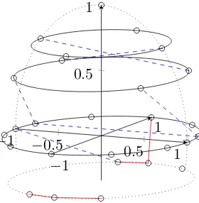
It is reasonable to suspect some intrinsic correlation of EEG sensors, e.g. due to position. To quantify and in-vestigate this we make use of our stochastic approach at hand. The correlation between sensor i and sensor j is ρij = Corr(Si, Sj). This correlation is readily computed
since we have a Legendre Chaos, which enables us to write the correlation in terms of the chaos expansion coefficients as
ρij=
P7,7
k=1VikVjk
q P7,7
k=1Vik2
q P7,7
k=1Vjk2
[image:3.595.77.267.336.508.2] [image:3.595.324.530.471.580.2]In Fig. 6 the sensorsiandj are connected by a blue dashed line if 0 ≤ |ρij| < .02, they are connected by a red solid
line if .9 ≤ |ρij|< 1. We observe high correlations in the
temporal region. It is apparent that the sensors in the occipital and lower frontal region, which are close together, are not so highly correlated as in the temporal regions. We note that we are dealing with overall mean sensor correlation, i.e. for averaged out dipole location, moment and conductivity ratio.
−
1
−
0
.
5
0
.
5
1
−
1
1
0
.
5
1
Figure 6. Visualization of correlation analysis. If0≤ |ρij|< .02then
sensoriis connected with sensorjby a blue dashed line. If.9≤ |ρij|<1
then sensoriis connected with sensorjby a red solid line.
We remind that it were also these sensors that are on average most influenced by a change in the conductivity ratio, see Fig. 2. When solving the inverse problem – of locating a dipole when sensor measurements are at hand – one needs to take these results into account: temporal sensors are highly correlated and highly sensitive to the conductivity ratio. E.g., one can give them less weight or try to minimize their influence in the solution of the inverse problem. Ideally a real time sensitivity and correlation analysis is combined with the techniques used to address the inversion.
Explaining this results qualitatively is a next step, where expert medical judgement, physiological and anatomical ex-pertise are required. This will be dealt with in the near future, being part of a interdisciplinary project.
IV. CONCLUSION
We discussed the modeling of the stochastic propagation of uncertain conductivity in EEG. Polynomial Chaos is intro-duced in the sensitivity and correlation analysis of the sensors influenced by uncertain conductivity. The analysis was con-ducted on a three layer spherical head model. We addressed the sensitivity analysis at three stages: dipole location and moment averaged out, only the dipole moment averaged out, and both fixed. On average, we observe the least influenced electrodes along the great longitudinal fissure. We compared two different source locations and obtained changes in the electrodes sensitivity, which we belief, are consistent with our intuitive hypothesis. The highly influenced sensors were on average located temporal. This was also the case in the correlation analysis. Sensors in the temporal parts of the brain are highly correlated. Whereas the sensors in the occipital
and lower frontal region, though they are close together, are not so highly correlated as in the temporal regions.
We hope this effective quantification of sensitivity and correlation can be useful in the EEG inverse problem, where iteratively the least influenced/correlated sensors are given more weight in the inverse algorithm. We are now trying to also make some sensor locations random and look for optimal placing of these sensors. Also, a more realistic head model and anisotropic conductivity distributions are a natural next topic of investigation [8].
Collaboration with researchers specifically dealing with practical EEG applications in medical investigations, will be set up in the frame of an interdisciplinary project between engineers, physicians and mathematicians. We continuously aim at contributing to the improvement of the reliability of the interpretation and use of the EEG-results in medical prognoses and remediation. We hope to report on this further research in a future WCE.
ACKNOWLEDGMENT
The author would like to thank the department of Electrical Energy, Systems and Automation (EESA) at Ghent
Univer-sity, and in particular Guillaume Crevecoeur, for providing the basis of a computer algorithm to compute the lead field. His office colleague Tine Goessens and colleague Hilde De Ridder are thanked for the fruitful discussions. His supervisors Roger Van Keer and Mari´an Slodiˇcka are thanked for their support.
REFERENCES
[1] M. Nolan, M. Redoblado, S. Lah, M. Sabaz, J. Lawson, A. Cunning-ham, A. Bleasel, and A. Bye, “Memory function in childhood epilepsy syndromes,”Journal of Paediatrics and Child Health, vol. 40, pp. 20–
27(8), January 2004.
[2] H. Urbach, “Imaging of the epilepsies,”European Radiology, vol. 15,
pp. 494–500, 2005.
[3] M. H¨am¨al¨ainen, R. Hari, R. Ilmoniemi, J. Knuutila, and O. V. Lounasmaa, “Magnetoencephalography—theory, instrumentation, and applications to noninvasive studies of the working human brain,”Rev. Mod. Phys., vol. 65, no. 2, pp. 413–497, Apr 1993.
[4] N. von Ellenrieder, C. Muravchik, M. Wagner, and A. Nehorai, “Effect of head shape variations among individuals on the EEG/MEG forward and inverse problems,” Biomedical Engineering, IEEE Trans. on,
vol. 56, no. 3, pp. 587 –597, mar. 2009.
[5] J. de Munck, B. van Dijk, and H. Spekreijse, “Mathematical dipoles are adequate to describe realistic generators of human brain activity,”
Biomedical Engineering, IEEE Trans. on, vol. 35, no. 11, pp. 960
–966, nov. 1988.
[6] L. Geddes and L. Baker, “The specific resistance of biological material–A compendium of data for the biomedical engineer and physiologist,” Medical and Biological Engineering and Computing,
vol. 5, pp. 271–293, 1967.
[7] S. Goncalve, J. de Munck, J. Verbunt, R. Heethaar, and F. da Silva, “In vivo measurement of the brain and skull resistivities using an EIT-based method and the combined analysis of SEF/SEP data,”
Biomedical Engineering, IEEE Trans. on, vol. 50, no. 9, pp. 1124
–1127, sep. 2003.
[8] C. Wolters, A. Anwander, X. Tricoche, D. Weinstein, M. Koch, and R. MacLeod, “Influence of tissue conductivity anisotropy on EEG/MEG field and return current computation in a realistic head model: A simulation and visualization study using high-resolution finite element modeling,”NeuroImage, vol. 30, no. 3, pp. 813 – 826,
2006.
[9] S. Vallaghe and M. Clerc, “A global sensitivity analysis of three- and four-layer EEG conductivity models,”Biomedical Engineering, IEEE Trans. on, vol. 56, no. 4, pp. 988 –995, apr. 2009.
[10] S. Cavassila, S. Deval, C. Huegen, D. van Ormondt, and D. Graveron-Demilly, “Cram´er-Rao bounds: an evaluation tool for quantitation,”
[image:4.595.98.238.193.336.2][11] A. Dogandzic and A. Nehorai, “Estimating evoked dipole responses in unknown spatially correlated noise with EEG/MEG arrays,”Signal Processing, IEEE Trans. on, vol. 48, no. 1, pp. 13 –25, jan. 2000.
[12] H. M. Huizenga and P. C. M. Molenaar, “Equivalent source estimation of scalp potential fields contaminated by heteroscedastic and correlated noise,”Brain Topography, vol. 8, pp. 13–33, 1995.
[13] N. Gencer and C. E. Acar, “Sensitivity of EEG and MEG measure-ments to tissue conductivity,”Physics in Medicine and Biology, vol. 49,
no. 5, p. 701, 2004.
[14] S. Rush and D. Driscoll, “EEG electrode sensitivity - An application of reciprocity,”Biomedical Engineering, IEEE Trans. on, vol. 16, no. 1,
pp. 15 –22, jan. 1969.
[15] D. B. Geselowitz, “On bioelectric potentials in an inhomogeneous volume conductor,”Biophysical Journal, vol. 7, no. 1, pp. 1 – 11,
1967.
[16] J. Riera and M. Fuentes, “Electric lead field for a piecewise homoge-neous volume conductor model of the head,”Biomedical Engineering, IEEE Trans. on, vol. 45, no. 6, pp. 746 –753, jun. 1998.
[17] N. Wiener, “The homogeneous chaos,”American Journal of Mathe-matics, vol. 60, no. 4, pp. 897–936, 1938.
[18] D. Xiu and G. E. Karniadakis, “The Wiener-Askey Polynomial Chaos for stochastic differential equations,”SIAM J. Sci. Comput., vol. 24,
no. 2, pp. 619–644, 2002.