Finding an Optimal Solution of an Assignment
Problem by Improved Zero Suffix Method
Neetoo Kardam1, Prof. R.B. Singh2
1
Student, 2Assistant Professor, Department of Mathematics, Monad University Hapur, India
Abstract: In this paper improved Zero Suffix Method is applied for finding an optimal solution for assignment problem. This method requires least iterations to reach optimality, compared to the existing methods available in the literature. Here numerical examples are solved to check the validity of the proposed method.
Keywords: Assignment Problem, Optimal Solution, Operation Research Problem, Cost minimization Assignment problem, improved Zero suffix method.
I. INTRODUCTION
The assignment problem is one of the earliest applications and is a special case of Operation Research problem, which deals with available sales-force to different regions: vehicles to toutes; products to factories; contracts to bidders; machines to jobs; development engineering to several construction sites and so on. Since all supplies, demands, and bounds on variables are integral, the assignment problem relies on a nice property of transportation problems that the optimal solution will be entirely integral. As you will see, the goal of the objective of the assignment problem ( unlike transportation problems) may not have anything to do at all with moving anything. Generally the management makes assignment on a one-to-one basis in such a manner that the group maximizes the revenue from the sales; the vehicles are deployed to various routes in such a way that the assignment cost is minimum and so on. Applications of assignment problems are varied in the real world. Certainly it can be useful for the classic task of assigning employees to tasks or machines to production jobs, but its uses are more widespread. It could be used to assign fleets of aircrafts to particular trips, or assigning school buses to toutes, or networking computer. In rare cases, it can even be used to determine marriage partners. A considerable number of methods have been so far presented for assignment broblem in which the Hungarian method is more convenient method among them. Different methods have been presented for transportation problem and various articles have been published on the subject. Many of the authors (1) – (3) have done the transportation problems in different methods. Pandian and Natarajan (4) proposed new method for finding an optimal solution directly for method respectively. The more for less method to distribution related problems was established by (7).
By a complete assignment for a cost matrix n x n, we mean an assignment plan containing exactly n assigned imdependent zeros, one in each row and one in each column. The main concept of assignment plan is optimal if optimizes the total cost or effectiveness of doing all the jobs.
Hence we applied new method named improved zero suffix method, which is defferent from the preceding methods to apply in the assignment problems.
II. IMPROVED ZERO SUFFIX METHOD
The working rele of finding the optimal solution is as follows:
1) Step 1: Construct the assignment problem.
2) Step 2: Subtract each row entries of the assignment table from the row minimum element.
3) Step 3: Subtract each column entries of the assignment table from the column minimum element.
4) Step 4: In the reduced cost matrix there will be at least one zero in each row and column, and then find the suffix value of all the zers in the reduced cost matrix by following simplification, the suffix value is denoted by S.
S=
And if the zeros lie in the same row or column then assign the job to that person whose cost is minimum. Now create a new assignment table by deleting that row & column which has been assigned.
6) Step 6: Repeat step 2 to step 3 until all the tasks has not been assigned to the persons.
A. Examples
1) Consider the following cost minimization assignment problem
J1 J2 J3 J4
B1 15 11 13 15
B2 17 12 12 13
B3 14 15 10 14
B4 16 18 11 17
Solution: On applying row minimum operation we get
J1 J2 J3 J4
B1 4 0 2 4
B2 5 0 0 1
B3 4 5 0 4
B4 5 7 0 6
Again on applying column minimum operation we get
J1 J2 J3 J4
B1 0 0 2 3
B2 1 0 0 0
B3 0 5 0 3
B4 1 7 0 5
Now find the suffix value of each element whose value is zero & write the suffix value within the bracket ( ). The suffix value is calculated by using the formula
S
J1 J2 J3 J4
D1 D2 D3 D4
B1 0 (2.3) 0 (5.6) 2 3
B2 1 0 (3.25) 0 (0.6) 0 (4)
B3 0 (3.3) 5 0 (2.5) 3
B4 1 7 0 (5) 5
From all of the above suffix, 5.6 is the maximum so assign the job J2 to the person B1 Next delete the 1st row and 2nd column from the above table and apply the same process.
J1 J3 J4
B2 1 O(0.25) 0(4.5)
B3 0(2.5) 0(0.75) 3
B4 1 0(2) 5
J1 J3
B3 0(0.5) 0(0)
B4 1 0(0.5)
From the above table, it is clear that the job J1 should be assigned to the person B3 and the job J3 should be assigned to the person B4 Finally the assignments are as follows B1- J2, B2 – J4, B3 – J1, B4 – J3
& the minimum assignment cost = Rs (11 + 13 + 14 + 11) = Rs 49
2) Consider the following travelling salesman problem
O1 ∞ 30 0 24
O2 1 ∞ 10 0
O3 50 0 ∞ 28
O4 4 4 0 ∞
Solution: On applying row minimum operation we get
D1 D2 D3 D4
O1 ∞ 30 0 24
O2 0 ∞ 10 0
O3 49 0 ∞ 28
O4 3 4 0 ∞
Again on applying column minimum operation we get
D1 D2 D3 D4
O1 ∞ 46 16 40
O2 41 ∞ 50 40
O3 82 32 ∞ 60
O4 40 40 36 ∞
Now find out the suffix value of each element whose value is zero & write the suffix value within the bracket ( ). The suffix value is calculated by using the formula
S=
D1 D2 D3 D4
O1 ∞ 30 0(32) 24
O2 0(53) ∞ 10 0(41)
O3 49 0(111) ∞ 28
O4 3 4 36(8.5) ∞
From all of the above suffix, 111 is maximum, so assign the origin O3 to the Destination D2 Next delete the 3rd row and 2nd column from above table and repeat the same process
D1 D3 D4
O1 ∞ 0(17) 24
O2 0(13.5) 10 0(12)
O4 3 0(6.5) ∞
D1 D3 D4
O1 ∞ 0 24
O2 0 10 0
O4 3 0 ∞
From all of the above suffix, 17 is maximum, so assign the origin O1 to the Destination D3 Next delete the 1st row and 3rd column from above table and repeat the same process
D1 D4
O2 ∞ 0(28)
O4 0(28) 28
From the above table it is clear that O2 – D4, O4 – D1
The optimum assignment is O1 – D3, O2 – D4, O3 – D2, O4 – D1 & the minimum cost = Rs (16 + 40 + 32 + 40)
= Rs 128
III. CONCLUSION
The proposed algorithm carries systematic procedure, and very easy to understand. From this paper, it can be concluded that Improved zero suffix Method provides an optimal solution in fewer iterations, for the assignment problems. As this method consumes less time and is very easy to understand and apply, so it will be very helpful for decision makers.
REFERENCES
[1] A Edward Samuel and M. Venkatachalapathy, “Modified Vogel’s Approximation method for Fuzzy Transportation Problem”, Applied Mathematical
Science, Vol. 5, No. 28, pp. 1367-1372, 2011.
[2] NagarajBalakrishnan, “Modified Vogel’s Approximation Method for Unbalanced Transportation Problem”, Applied Mathematics Letters 3, pp. 9-11,
1990.
[3] A. Nagooragani, “Fuzzy Transporation problem, Proceedings of national Seminar on Recent Advancement in Mathematics, 2009.
[4] P. Pandian, and G. Natarajan, “A new method for finding an optimal solution for Transportation problem,” International Journal of Mathematical Sciences
and Engineering Applications, Vol. 4, pp. 59-65, 2010.
[5] V. J. Sudhakar, N. Arunsankar, and T. Karpagam, “A New approach for finding an optimal Solution for transportation problem”, Applied European
Journal of Scientific Research, Vol.68, pp. 254-257,2012.
[6] Abdul Quddoos, ShakeelJavaid, and M. M. Khalid, “A New method for finding an Optimal Solution for Transportation Problem”, International Journal
on Computer Science and Engineering, Vol.4, No.7, July 2012.
[7] VeenaAdlakha, and Krzysztof Kowalski, “A heuristic method for mor-for less in distribution related problems”, Internal Journal of Mathematical
Education in Science and Technology, Vol. 32, pp. 61-71, 2001.
[8] H.A. Taha, Operations Research- Introduction, Prentice Hall of India, New Delhi, 2004.
[9] J. K. Sharma, Operations Research- Theory and applications, Macmillan India LTD, New Delhi, 2005.
[10] KantiSwarup, P. K. Gupta and Man Mohan, Operations Research, Sultan Chand & Sons, 12th Edition, 2004.
I. DEFINITION
The transportation problem is a special type of linear programming problem, where the objective is to minimize the cost of distributing a product from a number of sources to a number of destinations.
The gereral mathematical model may be given as follows
If xij (≥0) is the number of units shipped from ith source to jth destination, then equivalent LPP model will be Minimize Z=∑ ∑
Subject to
∑ ≤ For i = 1,2, ……, m (supply) ∑ ≤ For j = 1,2, ……, n (demand) Xij ≥0
For a feasible solution to exist, it is necessary that total capacity equals total to the requirements. If ∑ 1=∑ i.e. If total supply = total demand then it is a balanced transportation problem otherwise it is called unbalanced Transportation problem. There will be (m + n – 1) basic independent variables out of (m x n) variables
What are the understanding assumptions?
1) Only a single type of commodity is being shipped from an origin to a destination.
2) Total supply is equal to the demand.
∑ = ∑ , ai (Supply) and bj (demand) are all positive integers.
3) The unit transportation cost of the item from all sources to destinations is certainly and preciously known.
4) The objective is to minimize the total cost.
II. NORTH WEST CORNER RULE
1) Example 1: The ICARE Company has three plants located throughout a state with production capacity 50, 75 and 25 gallons. Each day the firm must furnish its four retail shops R1, R2, R3, & R4 with at least 20, 20, 50, and 60 gallons respectively. The transportation costs (in Rs.) are given below.
Company Retail Supply
R1 R2 R3 R4
P1 3 5 7 6 50
P2 2 5 8 2 75
P3 3 6 9 2 25
Demand 20 20 50 60
The economic problem is to distribute the available product to different retail shops in such a way so that the total transportation cost is minimum?
2) Solution: Starting from the North West corner, we allocate min (50, 20) to P1,R1 i.c., 20 unit to cell P1R1. The demand for the first column is satisfied. The allocation is shown in the following table.
Table 1
Company Retail Supply
R1 R2 R3 R4
P1 3 5 7 6 50
P2 2 5 8 2 75
P3 3 6 9 2 25
Demand 20 20 50 60
Now we move horizontally to the second column in the first row and allocate 20 units to cell P1R2. The demand for the second column is also satisfied.
2 2 1
4 3
Proceeding in this way, we observe that P1R3 = 10, P2R4 = 35, P3R4 = 25. The resulting feasible solution is shown in the following table.
Here, number of retail shops (n) = 4, and
Number of plants (m) = 3. Number of basic variables = m + n – 1 = 3 + 4 – 1 = 6.
A. Initial Basic Feasible Solution
The initial basic feasible solution is x11 = 20, x12=5, x13=20, x23=40, X24=35, X34=25 and minimum cost of transportation=20 X 3 + 10 X 7 + 40 X 8 + 35 X 2 + 25 X 2 =670
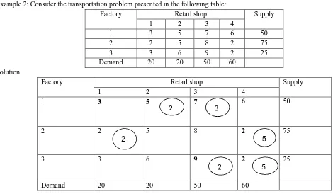
III. MATRIX MINIMUM METHOD Example 2: Consider the transportation problem presented in the following table:
Factory Retail shop Supply
1 2 3 4
1 3 5 7 6 50
2 2 5 8 2 75
3 3 6 9 2 25
Demand 20 20 50 60
Solution
Factory Retail shop Supply
1 2 3 4
1 3 5 7 6 50
2 2 5 8 2 75
3 3 6 9 2 25
Demand 20 20 50 60
Number of basic variables = m + n – 1 = 3 + 4 – 1 = 6.
A. Initial Basic Feasible Solution
The initial basic feasible solution is X12=20, X13=30, X21=20, X24=55, X233=20, X34=5 and minimum cost of transportation=20 X 2 + 20 X 5 + 30 X 7 + 55 X 2 + 20 X 9 + 5 X 2 = 650
B. Vogel Approximation Method (VAM)
The Vogel approximation (Unit penalty) method is an iterative procedure for computing a basic feasible solution of a transportation problem. This method is preferred over the two methods discussed in the previous sections, because the initial basic feasible solution obtained by this method is either optimal or very close to the optimal solution.
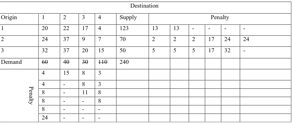
Example 3: Obtain an Initial BFS to the following Transportation problem using VAM method?
Origin Destination Supply
1 2 3 4
1 20 22 17 4 120
2 24 37 9 7 70
3 32 37 20 15 50
Demand 60 40 30 110 240
Solution: Since ∑ = ∑ , the given problem is balanced TP., Therefore there exists a feasible solution.
2 3
2
5
1) Step 1: Select the lowest and next to lowest cost for each row and each column, then the difference between them for each row and column displayed them with in first bracket against respective rows and columns. Here all the differences have been shown within first compartment. Maximum difference is 15 which is occurs at the second column. Allocate min (40, 120) in the minimum cost cell (1,2).
[image:7.612.70.549.167.371.2]2) Step 2: Appling the same techniques we obtained the initial BFS. Where all capacities and demand have been exhausted
Table Initial basic Destination
Origin 1 2 3 4 Supply Penalty
1 20 22 17 4 123 13 13 - - - -
2 24 37 9 7 70 2 2 2 17 24 24
3 32 37 20 15 50 5 5 5 17 32 -
Demand 60 40 30 110 240
P
e
na
lty
4 15 8 3
4 - 8 3
8 - 11 8
8 - - 8
8 - - -
24 - - -
C. Feasible solution
The initial basic feasible solution is X12=40, X14=40, X21=10, X23=30, X24=30, X31=50. and minimum cost of transportation=22 X 40 + 4 X 80 + 24 X 10 + 9 X 30 + 7 X 30 + 32 X 550 = 3520.
D. Optimality Test for Transportation Problem
There are basically two methods
a) Modified Distribution Method (MODI
b) Stepping Stone Method.
E. Modified Distribution Method (MODI)
The modified distribution method, also known as MODI method or (u – v) method provides a minimum cost solution to the transportation problem. In the stepping stone method, we have to draw as many closed paths as equal to the unoccupied cells for their evaluation. To the contrary, in MODI method, only closed path for the unoccupied cell with highest opportunity cost is drawn. Steps
1) Determine an initial basic feasible solution using any one of the three methods given below:
a) North West Corner Rule
b) Matrix Minimum Method
c) Vogel Approximation Method
2) Determine the values of dual variables, ui and vj, using ui + vj = cij
3) Compute the opportunity cost using ij = cij – ( ui + vj).
4) Check the sign of each opportunity cost.
a) If the opportunity costs of all the unoccupied cells are either positive or zero, the given solution is the optimal solution. On the other hand,
b) If one or more unoccupied cell has negative opportunity cost, the given solution is not an optimal solution and further savings in transportation cost are possible.
6) Draw a closed path or loop for the unoccupied cell selected in the previous step. Please note the right angle turn in this path is permitted only at occupied cells and at the original unoccupied cell.
7) Assign alternate plus and minus signs at the unoccupied cells on the corner points of the closed path with a plus sign at the cell being evaluated.
8) Determine the maximum number of units that should be shipped to this unoccupied cell. The smallest value with a negative position on the closed path indicates the number of units that can be shipped to the entering cell. Now, add this quantity to all the cells on the corner points of the closed path marked with plus signs, and subtract it from those cells marked with closed path marked with plus signs, and subtract it from those cells marked with minus signs. In this way, an unoccupied cell becomes an occupied cell.