Evaluation of Soil Erosion Status of Flatland
Micro-Watershed under Semi-Arid Conditions
using MMF Model
Shruti Shivaraj1, Nagraj S Patil2, Umapathy Satishkumar3, Rajesh Neralikere4
2
Ph.D., Associate Professor,1, 3, 4Dept.of Water and Land Management, Visvesvaraya Technological University, Belagavi 590018, Karnataka, India.
Abstract: The semi-arid areas are considered to be very sensitive areas where the soil with little or no vegetation are exposed to short duration and high intensity precipitation leading to the occurrence of physical and chemical processes by soil erosion and further resulting into soil degradation. A study was conducted to observe soil erosion using Morgan-Morgan-Finney (MMF) model (for soil loss) in Patapur Micro-Watershed of Manvi Taluk in Raichur District, Karnataka, India. Remote sensing satellite data were used to create the land use/land cover maps, which in turn were used to create the Effective Hydrologic Depth (EHD), Crop Cover (CC), Plant Height (PH), Annual Interception (A), Ratio of actual [Et] to potential [Eo] evapotranspiration (Et/Eo) and Plant Cover Management factor (C) maps. Slope map was created by using Digital Elevation Model (DEM) map which in turn was used to create slope map of the area, and also soil data were used to generate maps of soil related parameters. Absence of vegetation or forest, unscientific agricultural practices are the main reasons for the soil loss taking place in the study area. The MMF model simulated 85.05 mm of runoff and 0.176 kg/m2 of average transport capacity of soil particles due to runoff; the observed values were set to 108.15 mm and 0.184 kg/m2 respectively. The average soil detachment rate by raindrop impact was observed to be 1.77 kg/m2 by the model. The model estimated lowest and highest values of soil detachment by overland flow taking place in the study area ranges from 0.010 to 0.766 kg/m2, and that of soil detachment by raindrop impact ranges from 0.468 to 6.386 kg/m2. Model evaluation was performed by using percent difference (D), and value obtained by the same is -4.48%. Hence, introducing appropriate procedures based on the erosion severity predicted by MMF model in the catchment is vital for management of sustainable natural resources.
Keywords: erosion modelling, GIS, MMF model, semi-arid, transport capacity.
Citation: Shivaraj, S., Patil, N. S., Satishkumar, U., Neralikere, R (2019). Evaluation of Soil Erosion Status of Flatland Micro-Watershed under Semi-Arid Conditions using MMF Model. International Agricultural Engineering Journal, 28
I. INTRODUCTION
Soil erosion is the phenomenon of detachment of particles from one source, and transportation to an accumulation site, which is distant from the source point of detachment. Soil erosion is a sinister process and not easily identifiable by the farmers, up until the effects are severe and irreversible. Erosion is an unbalanced process which includes precipitation, topography, land use/land cover, soil texture, human activities and other factors that affect the soil beyond reasoning. These factors account for 70% to 90% of the total soil loss. Nonetheless, soil loss prediction is a tough process and it involves many elements.
Soil loss models such as Universal Soil Loss Equation (USLE), Revised Universal Soil Loss Equation (RUSLE), Modified Universal Soil Loss Equation (MUSLE), Morgan, Morgan and Finney (MMF), Water Erosion Prediction Project (WEPP), Annualized Agricultural Non-Point Source (AnnAGNPS), European Soil Erosion Model (EUROSEM), Soil and Water Assessment Tool (SWAT), Areal Non-point Source Watershed Environment Response Simulation (ANSWERS), etc. have been developed. As compared to these models, the MMF model retains the simplicity of USLE and was developed to predict soil loss annually in field sized plots on the hill slopes. Also, this model is a mixed model (physical –based empirical model), and requires less data than the other soil loss prediction models. The model uses 12 operating functions with 19 input parameters.
Soil erosion models need data such as topography, climate, soil type and properties, land use, soil depth, etc., to calculate the soil erosion. These models use GIS tools to know the spatial distribution of soil erosion in an area or region. GIS tools are used to generate the maps and also to know the status of the input parameters.
and the people living in this micro-watershed mainly practice agriculture. Therefore, the need is to not only compute the soil erosion rates but also to assess the amount of soil loss, thereafter increasing the productivity of the agricultural lands to apply soil conservation measures in case of severe erosion as the study area usually has a high temperature in summers and agriculture becomes hectic in the area.
The research approach of this study consists of four main steps: (a) To quantify the geomorphological characteristics of the selected Micro-Watershed, (b) To study the land use/land cover of Micro-Watershed, (c) To estimate the rate of soil loss using MMF model, and (d)Validation of the model by using the field measured data.
II. MATERIALS AND METHODS A. Study Area
The Patapur Micro-Watershed (as shown in Fig 1), is a typical micro-watershed system under semi-arid agro-climatic system having an area of 454.5 hectares. This micro-watershed is located 63 kilometres away from the Raichur district in Karnataka State, India. The study area lies between the Lat- 16˚ 07' 35.9'' and Long- 76o 51′ 33.3'' and Lat- 16˚ 08′ 22.3’’ and Long- 76˚ 53′ 27.7'' with an average elevation of 447 m above the mean sea level (MSL). The mean annual temperature of this area is 29oC and annual rainfall is 600 mm ; the relative humidity during monsoon is about 75% (Karnataka State Natural Disaster Monitoring Centre (KSNDMC), Bangalore). Cotton and pigeon pea are the major crops grown in the micro-watershed. The study area has an SMS (Silt Monitoring Station) installed in the micro-watershed (as shown in Fig. 2), as to learn about the soil erosion rates.
Fig. 1 Patapur Micro-Watershed, Manvi Taluk, Raichur, Karnataka
Fig. 2 Synoptic view of Silt Monitoring Station established in Patapur Micro-watershed.
B. MMF input parameters
The input parameters in the MMF model mainly involve rainfall data, soil data, slope data and vegetation data of the study area. The rainfall data involve the mean annual rainfall (R), intensity of erosive rain (I) and number of rainy days (Rn). The annual rainfall
data of Kavital village (which is 13 kilometres from the study area) were collected from the Karnataka State Natural Disaster Monitoring Centre (KSNDMC), Bangalore; and the intensity of erosive rainfall was taken as suggested by Morgan, Morgan & Finney (1984) i.e. 25 mm/hr for tropical climates. The soil data includes soil moisture content at field capacity (MS, % by weight), bulk density (BD, Mg/m3), cohesion of soil (COH) and soil erodibility index (K, gm/J). COH was found out using the torvane device. Soil texture also plays a very important role in the calculation of the soil data. The vegetation data involve annual interception (A), Effective Hydrological Depth (EHD), ratio of actual to potential evapotranspiration (Et/Eo), crop cover
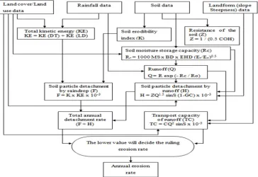
The study involved the use of MMF model as per Morgan, Morgan &Finney (1984), for the estimation of annual rate of soil erosion using GIS techniques. The flow chart showing the methods used in the execution of the model and it is shown in Fig. 3.
Fig. 3. Flowchart depicting Morgan- Morgan-Finney model of runoff and soil loss.
C. Soil Analysis
The micro-watershed was divided into 29 different mapping units based on physiography and landforms of the area and geomorphological characteristics such as slope, surface stoniness, erosion, drainage and gravelliness. Eighteen soil profiles were studied for soil depth, texture, colour, consistency, post fragments, etc. Soil samples were collected in October 2016 from these areas and soil particle analysis was carried out using International Pipette Method. The soil samples were tested in laboratory for particle size classification using this method, which used Stoke’s law and particle size classification- and was done based on the USDA standards. Soil moisture content at field capacity (MS) was calculated by the gravimetric method of calculation of soil moisture content at field capacity by oven drying. BD was calculated as per the core-sampler method.
D. Model Equations in the Execution of MMF model
The MMF model divides the soil erosion process into water phase and sediment phase; and their formulae are as follows:
1) Water Phase
ER = R x (1-A) ... (1)
DT = ER-LD ... (2)
LD = ER x CC ... (3)
KE (DT) = DT (11.9+8.7 log (I)) ... (4)
KE (LD) = (15.8 x PH0.5)-5.87 ... (5)
KE = KE (DT) + KE (LD) ... (6)
Q = R exp x (-Rc/Ro) ... (7)
Where, Rc = 1000 x MS x BD x EHD x (Et/Eo)0.5 Ro = R/ Rn 2) Sediment Phase F = K x KE x10-3 ... (8)
H = ZQ1.5 x sin S (1-GC) x 10-3 ... (9)
Where, LD is leaf drainage (mm). ER is effective rainfall (mm). CC is crop/canopy cover. Q is volume of overland flow (mm). Et/Eo
is ratio of actual to potential evapotranspiration. K is soil erodibility index (gm/J). F is the rate of soil detachment by raindrop impact (kg/m2). Z is resistance of soil. GC is ground cover. His rate of soil detachment by runoff (kg/m2). J is the rate of total soil particle detachment (kg/m2). G is the transport capacity of overland flow (kg/m2). The overall time required to acquire the data for this model was 12 weeks.
E. Application of GIS technique
After the study of the input parameters and their calculations, the data were entered in ArcGIS 10.4 and maps of these input parameters were generated at RS and GIS lab, Sujala-III project of Agricultural College, UAS Raichur. Kriging method was used for the map generation of some of the input parameters.
F. Statistical analysis
Statistical analysis was carried out for this study whereas; validation was carried out by using the model evaluation equation and getting the percentage difference. Sensitivity analysis was done for nine events of rainfall by changing the sensitive parameter values within the range and then observing the output of soil loss. It is an evaluation of the relative magnitude of change in the model response as a function of relative changes in the values of model input parameters (Nearing et al, 1990).
The sensitivity analysis was done by using the equation as shown below.
s = [(O2 –O1) /O12] / [(I2-I1) / I12] ... (12)
Where, s = sensitivity ratio of an input parameter, I1, I2 and O1, O2 = least and greatest values of the input and output parameters
respectively, and I12 and O12 = average of two inputs and outputs respectively.
G. Model Evaluation
The percent difference ( ) was used as a method for suitable measure of model prediction. The model estimated soil loss rate in this study was evaluated with respect to the sediment deposited surveyed in the reservoir. measured the average difference between the simulated and measured values as
... (13)
Where, p is the model simulated value, q is the observed soil loss value, and D is the percentage difference. A value nearer to 0% is considered the best for percentage difference, but higher values of D if the accuracy of gathered observed data is relatively low (Chekol, 2006).
III. RESULTS AND DISCUSSIONS
The study was carried out in the year of 2016 with 29 different mapping units and with different soil characteristics. R for the year of 2016 was found to be 843.8 mm and Rn was 39 days. The intensity of rainfall was taken as given by Morgan, Morgan & Finney
(1984) i.e. 25 mm/hr. The very steep slope was found to be 25% which is 14.32°. Slope map is as seen in Fig. 3 (a).
The bulk density of top soil went as high as 1.38 mg/m3, which had a slope of 10% and soil texture sandy clay was with poor vegetation cover. The bulk density was as low as 1.18 mg/m3 which had a slope of 3% and had clay as soil texture and cotton crop as vegetation cover. An increase in the bulk density affected the soil circulation by air, water, root systems and plant nutrients, and thus increased the rate of soil erosion. The soil moisture at field capacity revealed that it was as high as 0.45% by weight for the clay soil texture and as low as 0.25% by weight for sandy loam soil texture. The MS also decreased in case of a low soil quality, deprived land management practices, etc. EHD was used in the study as per the typical values given by Morgan, Morgan & Finney (1984) for the MMF method. It was revealed that the EHD was high on open scrubs and for the crop covered areas by pearl millet. Overall, EHD varied from 0.10 to 0.16 m. No terracing was done in the study area so as to affect the values of the EHD of the study area. The Et/Eo was found to range from 0.62 to 1.02, the higher values (0.67- 1.02) showed the vegetation to be cotton, open scrub,
cultivated grass or paddy crops; the lower values (0.62-0.67) showed the vegetation to be pearl millet or cotton. The evapotranspiration ratio was found to be more for an open scrub land than the cultivated areas. The crop cover management factor (C) ranged from 0.05 to 0.90, the lesser of which is for the growth of grass and the highest of which is for pearl millet as seen in Fig 3 (h). Areas with a higher C value are seen to have lower Et/Eo values and vice-versa.
The soil moisture storage capacity (Rc) is the function of MS, BD, EHD and Et/Eo, and this varies from 30.48 to 70.92. Most of the
of Rc value were seen in an area of steep slope percentage, i.e. 25% sloping. Normally, low Rc values indicate high runoff and these
soils are vulnerable to soil detachment by raindrop or by runoff. Low EHD also means low Rc, which leads to high runoff.
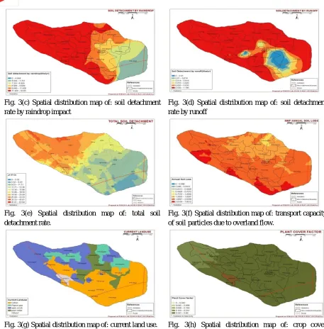
The soil detachment due to runoff (H) requires the understanding the input parameters of COH, using which Z is calculated. Also, the fraction of GC, S and volume of overland flow (Q) are important parameters for the estimation of soil detachment due to runoff. K influences F. The K values range as high as 0.70 gm/J and as low as 0.05 gm/J. The K value was calculated using the international pipette method, using the coarse, fine and very fine sand, clay and silt percentages along with organic matter content and soil permeability. The soil loss estimation was done by comparing J and G. Total soil erosion rate comprises of F and H. From the spatial distribution map of soil detachment by rainfall impact in Fig 3 (c), it is understood that the soil detachment is more on the hilly as well as the flat areas. The raindrop impact on inclination is close to the flatland areas. The F values ranged between 4.68 and 63.68 kg/m2 in the study area. H increases with increase in the slope steepness and so increases the velocity of soil transport. From the spatial distribution map Fig 3. (d), it is understood that H was low on flatlands and very high on the sloping lands.
The H values ranged from 0.00040 to 0.11961 kg/m2. J was ranging from 0.47to 6.40 kg/m2. The spatial distribution map of J is as shown in Fig. 3 (e).
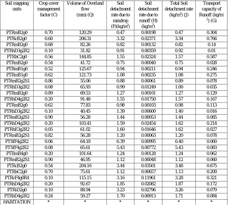
[image:5.612.73.542.311.731.2]G is governed by C, overland flow (Q) and the slope (S) of the area. G values ranged between 0.010 and 0.766 kg/m2 (or 0.10 tonnes/hectare/yr to 7.66 tonnes/hectare/yr) as seen in Fig. 3(f). Table. 1 shows the results of the MMF model.
Table 1 Crop cover management, volume of overland flow, rate of soil detachment by raindrop and runoff, total soil detachment rate and transport capacity of runoff values used in the model.
Soil mapping units
Crop cover management
factor (C)
Volume of Overland flow (mm) (Q)
Soil detachment
rate due to raindrop (F)(kg/m2)
Soil detachment
rate due to runoff (H) (kg/m2)
Total Soil detachment rate
(kg/m2) (J)
Transport capacity of Runoff (kg/m
-2 ) (G)
PTRmB2g0 0.70 120.29 0.47 0.00198 0.47 0.304
PTRcB2g0 0.60 206.31 3.32 0.02371 3.34 0.766
PTRmB2g0 0.68 82.26 0.82 0.00132 0.82 0.14
PTRhD3g2R2 0.10 31.82 0.91 0.00359 0.92 0.01
PTRhC2g0 0.56 144.85 1.55 0.02324 1.57 0.587
PTRmB2g0 0.54 41.72 0.75 0.00040 0.75 0.028
PTRmB1g0 0.52 125.67 0.94 0.00211 0.94 0.246
PTRmB1g0 0.62 121.73 1.08 0.00235 1.08 0.275
PTRmB2g2S1 0.86 55.06 0.88 0.00061 0.89 0.078
PTRhD3g2R2 0.08 65.93 0.99 0.01249 1.00 0.035
PTRmB2g0 0.89 69.53 1.27 0.00101 1.27 0.129
PTRhD4g2R2 0.20 91.48 1.55 0.01750 1.57 0.167
PTRmB2g0 0.62 77.83 0.98 0.00103 0.98 0.113
PTRhD3g2R2 0.10 40.45 1.39 0.00600 1.40 0.016
PTRmB2g2S1 0.90 56.28 1.44 0.00053 1.44 0.085
PTRhD4g2R2 0.20 103.41 1.59 0.02454 1.62 0.214
PTRhE3g2R2 0.05 61.02 1.60 0.01646 1.62 0.027
PTRmB2g2S1 0.82 56.28 1.20 0.00063 1.20 0.078
PTSfF4g2R2 0.06 64.18 6.39 0.00995 6.40 0.060
PTSfF4g2R2 0.08 65.61 5.43 0.00772 5.43 0.083
PTRmB4g0 0.20 101.64 1.24 0.00128 1.24 0.062
PTRmB2g2S1 0.90 46.95 1.12 0.00048 1.12 0.060
PTRcB2g0 0.54 204.16 3.44 0.03501 3.48 0.675
PTRhC2g0 0.70 75.61 1.12 0.00657 1.13 0.200
PTRcF4g0R4 0.10 115.15 3.16 0.11961 3.28 0.321
PTRhD4g2R2 0.20 92.67 1.85 0.02082 1.87 0.172
PTRiD2g0 0.10 88.94 3.23 0.02796 3.26 0.079
PTRhD4g2R2 0.24 59.27 1.70 0.00913 1.71 0.084
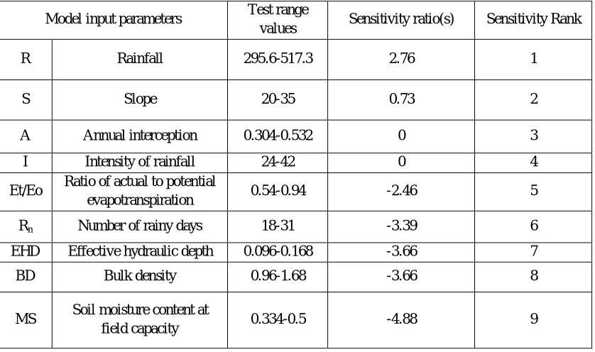
The sensitivity ratio ‘S’ was computed for the parameters of rainfall, slope, MS, BD, EHD, annual interception, Et/Eo and Rn. Sensitivity analysis was done by taking a base value. The lower input parameter values were taken 20% lower than the base value, and the higher input parameters were taken 40% more than the base value. This change was undertaken as the study area is a flatland in semi-arid conditions, and a slight change as small as ±10% would not cause a huge difference in the soil loss at the output. A negative value shows a decline in soil loss with increase in input parameter value.
Table 2 Sensitivity ratios of different input parameters for MMF model.
Model input parameters Test range
values Sensitivity ratio(s) Sensitivity Rank
R Rainfall 295.6-517.3 2.76 1
S Slope 20-35 0.73 2
A Annual interception 0.304-0.532 0 3
I Intensity of rainfall 24-42 0 4
Et/Eo Ratio of actual to potential
evapotranspiration 0.54-0.94 -2.46 5
Rn Number of rainy days 18-31 -3.39 6
EHD Effective hydraulic depth 0.096-0.168 -3.66 7
BD Bulk density 0.96-1.68 -3.66 8
MS Soil moisture content at
field capacity 0.334-0.5 -4.88 9
The MMF model does consider intensity indirectly in the form of KE which decides the erosive power of rainfall impact on different soils or soils with particular land use. Hence, though intensity of rainfall (I) mm/hr is a sensitive parameter, it is not determined so in the model. The values of sensitive input parameters are as shown in Table 2. The simulated rainfall energy and its rate help in deciding detachment of soil which is generally at higher rate rather than transportation capacity due to runoff. In the Patapur Micro-Watershed also, it has been experienced from data that runoff carrying capacity due to flatter slopes of the land and the carrying capacity of runoff of silt was lesser, even though sufficiently higher sediment was detached from a given place due to rainfall impact. The study reveals that, there is a need for protection/conservation measures to control moderate rainfall impact through contour bunding system, which not only minimizes effect of raindrop impact, but also helps to observe runoff at field scale level, sufficient enough to reduce sediment transportation to outlet.
Fig. 3(a) Spatial distribution map of: slope of the study area.
[image:6.612.83.524.549.699.2]Fig. 3(c) Spatial distribution map of: soil detachment rate by raindrop impact
Fig. 3(d) Spatial distribution map of: soil detachment rate by runoff
Fig. 3(e) Spatial distribution map of: total soil detachment rate.
Fig. 3(f) Spatial distribution map of: transport capacity of soil particles due to overland flow.
Fig. 3(g) Spatial distribution map of: current land use. Fig. 3(h) Spatial distribution map of: crop cover management factor.
IV. CONCLUSION
[image:7.612.73.530.67.531.2]V. ACKNOWLEDGEMENTS
This work would not be completed without the help of Dr. Nagraj. S. Patil, whose guidance and support influenced the accomplishment of the project, Dr. Umapathy Satishkumar and Dr. Rajesh Neralikere, whose constant encouragement and advice helped me have a deeper understanding of the subject and made me work hard on the project.
I would also like to thank Mr. Premanand. D, Dr. Ibrahim Khaleel and Dr. C. Sudharshan for their help during the project.
REFERENCES
[1] Ande, O.T., Alaga, Y., & Oluwatosin, G.A. (2009). Soil erosion prediction using MMF model on a highly dissected hilly terrain of Ekiti environs in southwestern Nigeria.International journal of Physical Sciences, 4(2), 53-57.
[2] Bohluli, M., The, C. B. S., Hanif, A. H. M., & Rahman, Z. A. (2015). Review on use of Silt Pits (Contour Trenches) as a soil and water conservation.Universiti Putra Malaysia Press, 3,63-80.
[3] Chandramohan, T., Venkatesh, B., &Balchand, A. N. (2015). Evaluation of three soil erosion models for small watersheds.International Conference on Water Resources, Coastal and Ocean Engineering, 4,1227-1234.
[4] Chekol. A. D. (2006), Modeling of hydrology and soil erosion of upper Awash river basin, Ethiopia, (Doctoral thesis, University of Bonn, Bonn, Germany). Retrieved from http://library.wur.nl/WebQuery/wda/1814679
[5] Ganasri, B. P., &Ramesh, H. (2016). Assessment of soil erosion by RUSLE model using remote sensing and GIS- A case study of Nethravathi Basin. Geoscience Frontiers,7(6), 953-961.
[6] Gelagay, H.S., &Minale, A. S. (2016). Soil loss estimation using GIS and Remote Sensing techniques: A case of Koga Watershed, Northwestern Ethiopia.International Soil and Water Conservation Research, 4(2), 126-136.
[7] Ghosh, S., &Guchhait, S.K. (2012). Soil loss estimation through USLE and MMF methods in the Lateritic Tracts of Eastern Plateau Fringe of Rajmahal Traps.Ethiopian Journal of Environmental Studies and Management, 5(4), 1-13.
[8] Golosov, V., &Belyaev, V. (2013).The history and assessment of effectiveness of soil erosion control measures deployed in Russia- International Soil and Water Conservation Research, 1(2), 26-35.
[9] Kartic Kumar. M., Annadurai R., and Ravichandran P.T (2014) Assessment of soil erosion susceptibility in Kothagiri taluk using RUSLE and geo-spatial technology- International Journal of scientific and research publications, volume 4(10), 1-13
[10] Laflen, J. M., &Flanagan, D. C. (2013). The development of U. S. soil erosion prediction and modeling.International Soil and Water Conservation Research, 1(2), 1-11.
[11] Li, C., Qi, J., Feng, Z., Yin, R., Guo, B., Zhang, F., & Zou, S. (2010). Quantifying the effect of ecological restoration on soil erosion in China’s Loess Plateau Region: An application of MMF approach.Environmental Management,45(3), 476-487.
[12] Mohamadi, M.A., &Kavian, A. (2015). Effects of rainfall patterns on runoff and soil erosion in field plots.International Soil and Water Conservation Research, 3(4), 273-281.
[13] Morgan R.P.C., (2005) “Soil Erosion and Conservation”, (3 Ed), (pp 129-137), Massachusetts, Blackwell publishing.
[14] Morgan, R.P.C.,&Duzant, J.H. (2008). Modified MMF (Morgan-Morgan-Finney) model for evaluating effects of crops and vegetation cover on soil erosion. Earth Surface Process and Landforms,33(1),90-106.
[15] Morgan, R.P.C., Morgan, D.D.V., & Finney, H.J. (1984). A predictive model for assessment of soil erosion risk. Journal of Agricultural Engineering Research, 30, 245-253.
[16] Morgan, R.P.C. (2001). A simple approach to soil loss prediction; a revised Morgan-Morgan-Finney model, CATENA, 44(4), 305-322.
[17] Panagos, P., Borrelli, P., Meusburger, K., Alewell, C., Lugato, E., &Montanarella, L.(2015). Estimating soil erosion cover-management factor at European scale.Land Use Policy, 48, 38-50.
[18] Panagos,P.,Borrelli,P.,Meusburger, K., Zanden,E. H. V. D., Poesen,J., &Alewell, C. (2015). Modelling the effect of support practices (P-factor) on the reduction of soil erosion by water at European scale.Environmental Science and Policy, 51, 23-34.
[19] Panagos,P., Borrelli,P., Meusburger, K., Zanden,E. H. V. D., Poesen, J., &Alewell, C. (2015). The new assessment of Soil loss by Water Erosion in Europe.Environmental Science and Policy, 54, 438-447.
[20] Prasannakumar,V.,Vijith, H., Abinod, S., &Geetha, N. (2012).Estimation of soil erosion risk within a small mountainous sub-watershed in Kerala, India, using Revised Universal Soil Loss Equation (RUSLE) and geo-information technology.Geoscience Frontiers,3(2),209-215.
[21] Shinde, V., Tiwari, K. N.,&Singh, M. (2010) Prioritization of micro watersheds on the basis ofsoil erosion hazard using remote sensing and geographic information system.International Journal of Water Resources and Environmental Engineering,2(3), 130-136.
[22] Singh, G., &Panda, R. K. (2017). Grid-cell based assessment of soil erosion potential for identification of critical erosion prone areas using USLE, GIS and remote sensing: A case study in the Kapgari watershed, India.International Soil and Water Conservation Research, 5(3),202-211.
[23] Tesfahunegn G.B., Tamene L., and Vlek P.L.G (2014), Soil erosion prediction using Morgan-Morgan-Finney model in a GIS environment in northern Ethiopia catchment- Applied and environmental soil science,( 2014, 1-15). Retrieved from https://www.hindawi.com/journals/aess/2014/468751/
[24] Vieira, D.C.S., Prats, S.A., Nunes, J.P., Shakesby, R.A., Coelho, C.O.A., & Keizer, J.J. (2014). Modelling runoff and erosion, and their mitigation, in burned Portuguese forest using revised Morgan-Morgan-Finney model- Forest Ecology and Management, 314, 150-165.
[25] Zhang, H., Wei, J., Yang, Q., Baartman, J. E. M., Gai, L., Yang, X., Li, S., Yu, J., Ritsema, C. J., &Geissen, V. (2017). An improved method for calculating slope length (λ) and the LS parameters of the Revised Universal Soil Loss Equation for large watersheds.Geoderma, 308,36-45.