Optimization of Machining Parameter on CNC Leadwell of SS304l by using Topsis Method

Optimization of Machining Parameter on CNC

Leadwell of SS304l by using Topsis Method

Shashank Rathore1, Nitin Shukla2

1

Department Of Mechanical Engineeing, Dr.C V Raman University Kota Bilaspur

Abstract: The main challenge in manufacturing industry is to optimize the energy consumption. Energy mainly consumes by machine tools in turning, drilling, boring processes, etc. The present work is to optimize the parameters cutting velocity, feed and depth of cut .while turning operation to maximize the material removal rate (MRR) and to minimize the surface roughness (SR) in a LEADWELL CNC MACHINE on AISI 304 austenitic stainless steel. Stainless steel has been chosen because it has unique properties like corrosion resistance, heat resistance, welding, Excellent weld ability by all standard fusion Heat Treatment etc. which can be taken advantage of in variety of applications in construction industries whilst at the same time being tough, hygienic, adaptable, and recyclable. Turning is one of the important and widely used machining processes in engineering industry. Experiments are design based on Taguchi orthogonal array and process parameters are optimized by using TOPSIS. Keywords: TOPSIS, SS304L.

I. INTRODUCTION

A. Turning

Turning is a machining process to produce parts round in shape by a single point tool on lathes. The tool is fed either linearly in the direction parallel or perpendicular to the axis of rotation of the work piece, or along a specified path to produce complex rotational shapes. The primary motion of cutting in turning is the rotation of the workpiece, and the secondary motion of cutting is the feed motion.

B. Stainless Steel Material

Iron and the most common iron alloy steel are, from a corrosion view point, relatively poor materials as they rust in air, corrode in acids and scale in furnace atmosphere. In spite of this there is a group of iron base alloys, the iron-chromium-nickel alloysknown as stainless steels, which are resistant to concentrated acids, alkalis and which do not scale under temperatures upto 1100˚C. The most widely used stainless steels are the austenitic 18/8 type steels, i.e. AISI 304 and AISI 304L, which form more than 50% of the global production of stainless steels. The next most widely used grades are the ferritic steels such as AISI 410 followed by the molybdenum-alloyed steels AISI 316 and AISI 316L. Together these grades make up over 80% of the total tonnage of stainless steels. Stainless steels with their excellent corrosion properties have a very broad application range. This extends to Chemical plants, Dairy and Food processing industries, Nuclear power plants, Heat exchangers, Laboratory benches and Equipments.

C. Sensitization Of Stainless Steels

In Sensitization process chromium carbides (Cr23C6) precipitate at the grain boundaries even atelevated temperatures, typically between 450 – 850° C. As a result, some chromium is lost and eventually reduces the corrosion resistance property of the Stainless steels4. This results in reduced ductility, toughness and aqueous corrosion resistance. Except the ‘L’ grade stainless steels all the other stainless steels are easily susceptible to sensitization.

TABLE 1.1COMPOSITION OF 304LSS

ALLOY GRADE C Mn P S Si Cr Ni Mo

304L 0.01 1.638 0.023 0.002 0.412 .18.56 8.138 0.364

D. Surface Integrity

In machining, a surface can be defined as a border between a machined component and its environment. The term ‘surface integrity’ is used to describe the attributes of a machined surface and its relationship to functional performance.

wear and lubrication, and dimensional accuracy). The surface integrity plays a very important role in this functional performance, being dependent of a large number of machining parameters. The major concern of the industry is to know which combination of machining parameters provides a better surface integrity of the machined components.

E. TOPSIS

Topsis (technique for order preference by similarity to ideal solution ) method was firstly proposed by (Hwang and Yoon 1981). Technique for Order Preference by Similarity to Ideal Solution• Yoon and Hwang introduced the TOPSIS method based on the idea that the best alternative should have the shortest distance from the positive ideal solution and farthest distance from the negativeideal solution. method are discussed in experimental procedure topic

F. Project Problem Definition

The objective of this work is to optimize the parameters cutting velocity, feed depth of cut while turning operation to maximize the material removal rate (MRR) and to minimize the power consumption (P), surface roughness(Ra) ,Micro hardness(HV) and cutting force (Fc) in a LEADWELL CNC MACHINE on AISI 304L austenitic stainless Steel.Optimisation process was done by TOPSIS of ranking approach.Application of regression analysis is used for finding the significant parameter.Model was developed using artificial neural network (ANN) algorithm to relate the responses with input variables

II. LITERATURESURVEY

Generally the Taguchi method is using to optimize the performance characteristics of process parameters to achieve high quality [1, 2]. However, reports on Taguchi have been concerned with the optimization of a single performance characteristic [3].So for the more demanding multiple performance characteristics is still an interesting research problem

A. Literature Survey On Regression Analysis

Ashok Kumar Sahoo and Swastik Pradhan (2013) this paper presents the influence of process parameters. They using TAGUCHI experiment design for experiment on different parameter and also used ANOVA and least square method is adopted in regression analysis to find the coefficients of equation. And they calculated predicted value of responses parameter [4].

Carmita Camposeco-Negrete (2013) he presented to optimize cutting parameters during Turning of AISI 6061 T6 under roughing conditions in order to get the minimum energy consumption. An orthogonal array, signal to noise (S/N) ratio and analysis of variance (ANOVA) and they concluded according to influence of factor in different cases . [5].

Debabrata Mandal et al. (2007) they using soft computing techniques. Artificial neural network (ANN) with back propagation algorithm is used to model the process and regration analysis [6].

Rajesh Kumar Bhushan (2013) they used response surface methodology. Face cantered central composite Design (FCCD) for three level design and experimentally collected data were subjected to ANOVA and desirability function analysis for optimization of machining parameters [9].

B. Literature Survey On Topsis

Ashvin J et al. (2013) in this paper, application of RSM on the AISI 410 steel is carried out for turning operation. A quadratic model has been developed for surface roughness (Ra) to investigate the influence of machining parameters. [11].

Hae-Sung Yoon et al. (2013) works related to the optimization of energy consumption of machine tools have been carried Control of machining parameters for energy and cost savings in Micro-scale drilling of PCBs [12] .

B. C. Rautara et al. (2012) works related to the optimization of energy consumption in this paper response surface methodology has been applied to determine optimum parameter of machining in cnc turning operation on EN 8 steel. And the machining was carried by coted carbide tool. [13].

III. OBJECTIVESOFPROJECTWORK

Objectives of study are as follows

A. To determine the optimum input parameter (speed, feed and depth of cut) for turning process on LEADWELL CNC to maximize the MRR and surface roughness.

B. To develop model by Regration analysis and study the turning process of stainless steel 304L on CNC.

IV. POSSIBLEOUTCOMES A. To get machining data

B. Optimization by TOPSIS

C. To get optimum parameter to get max MRR and low surface roughness.

V. EXPERIMENTALWORK

A. Experimental Setup

Vickers MicroHardness was measured on the surface at three location with 0.5kgf indentation using dwell time equal to 10 seconds of each sample.Cutting forces were measured by Kistler force dynamometer mounted on CNC bead .Turning tests were conducted with coated tungsten carbide inserts with an ISO designation CNMG 120404 was used. The inserts were mounted on a tool holder with an ISO designation PCLNL 1610 M12.

Fig 5.1 work piece material after turning

B.Material

SS304L of diameter 26 mm and cutting length 20mm

TABLE 5.1PHYSICAL PROPERTIES OF 304LGRADE STAINLESS STEEL

Density (kg/m3)

Density (kg/m3)

Elastic Modulus (GPa)

Mean Coefficient of Thermal Expansion

(μm/m/°C)

Thermal Conductivity (W/m.K)

Specific Heat 0-100°C (J/kg.K)

Electrical Resistivity

(nΩ.m)

304L 8000 193 100°C 315° C

538°C 100 °C

500 °C

500 720

17.2 17.8 18.4 16.2 21.25

C. Machine

LEADWELL CNC turning center with maximum speed of 4500 rpm

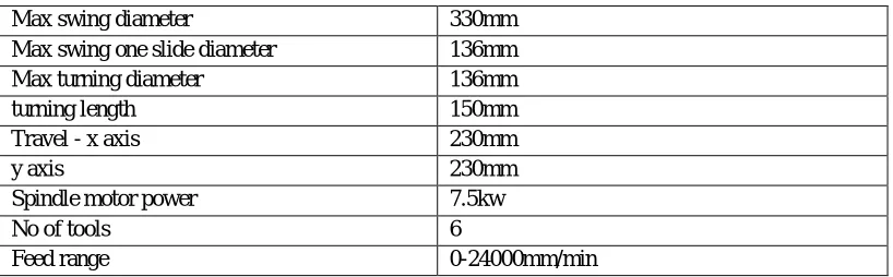
TABLE 5.2SPECIFICATION OF MACHINE

Max swing diameter 330mm Max swing one slide diameter 136mm Max turning diameter 136mm

turning length 150mm

Travel - x axis 230mm

y axis 230mm

Spindle motor power 7.5kw

No of tools 6

Feed range 0-24000mm/min

D. Experimental Parameter And Design

E. Experimental results

TABLE 5.3ORTHOGONAL DESIGN WITH EXPERIMENTAL RESPONSE VALUE

s. no. Speed Feed DOC Ra MRR

1 100 0.1 0.3 1.133 2.355

2 100 0.15 0.6 1.500 4.71

3 100 0.2 0.9 2.007 7.067

4 150 0.1 0.6 1.110 7.06

5 150 0.15 0.9 1.013 10.59

6 150 0.2 0.3 2.353 3.53

7 200 0.1 0.9 1.490 14.13

8 200 0.15 0.3 1.497 4.71

9 200 0.2 0.6 2.077 9.42

The most valuable use of regression is in making predictions. The general purpose of multiple regressions is to learn more about the relationship between several independent or predictor variables and a dependent or criterion variable.

It can be used for a variety of purposes such as analyzing of experimental, ordinal, or categorical data. The data presented in Table 4 have been used to build the multiple regression model

Exp. No speed feed doc Ra MRR

1 100 0.1 0.3 1.182763 1.76488

2 100 0.1 0.45 1.124452 3.530875

3 100 0.1 0.6 1.06614 5.29687

4 100 0.1 0.75 1.007829 7.062865

5 100 0.1 0.9 0.949518 8.82886

6 100 0.125 0.3 1.366666 1.47088

7 100 0.125 0.45 1.270649 3.236875

8 100 0.125 0.6 1.174633 5.00287

9 100 0.125 0.75 1.078616 6.768865

10 100 0.125 0.9 0.982599 8.53486

11 100 0.15 0.3 1.706608 1.17688

12 100 0.15 0.45 1.572886 2.942875

13 100 0.15 0.6 1.439164 4.70887

14 100 0.15 0.75 1.305442 6.474865

15 100 0.15 0.9 1.17172 8.24086

16 100 0.2 0.3 2.854609 0.58888

17 100 0.2 0.45 2.645476 2.354875

18 100 0.2 0.6 2.436342 4.12087

19 100 0.2 0.75 2.227209 5.886865

20 100 0.2 0.9 2.018076 7.65286

21 125 0.1 0.3 1.077916 2.942213

22 125 0.1 0.45 1.042733 4.708208

23 125 0.1 0.6 1.007549 6.474203

24 125 0.1 0.75 0.972366 8.240198

25 125 0.1 0.9 0.937182 10.00619

26 125 0.125 0.3 1.214747 2.648213

27 125 0.125 0.45 1.141858 4.414208

28 125 0.125 0.6 1.068969 6.180203

29 125 0.125 0.75 0.99608 7.946198

31 125 0.15 0.3 1.507616 2.354213

32 125 0.15 0.45 1.397022 4.120208

33 125 0.15 0.6 1.286428 5.886203

34 125 0.15 0.75 1.175833 7.652198

35 125 0.15 0.9 1.065239 9.418193

36 125 0.2 0.3 2.561472 1.766213

37 125 0.2 0.45 2.375467 3.532208

38 125 0.2 0.6 2.189461 5.298203

39 125 0.2 0.75 2.003456 7.064198

40 125 0.2 0.9 1.81745 8.830193

41 150 0.1 0.3 1.073275 4.119545

42 150 0.1 0.45 1.061219 5.88554

43 150 0.1 0.6 1.049163 7.651535

44 150 0.1 0.75 1.037108 9.41753

45 150 0.1 0.9 1.025052 11.18353

46 150 0.125 0.3 1.163033 3.825545

47 150 0.125 0.45 1.113272 5.59154

48 150 0.125 0.6 1.063511 7.357535

49 150 0.125 0.75 1.01375 9.12353

50 150 0.125 0.9 0.963988 10.88953

51 150 0.15 0.3 1.40883 3.531545

52 150 0.15 0.45 1.321364 5.29754

53 150 0.15 0.6 1.233897 7.063535

54 150 0.15 0.75 1.14643 8.82953

55 150 0.15 0.9 1.058963 10.59553

56 150 0.2 0.3 2.368541 2.943545

57 150 0.2 0.45 2.205663 4.70954

58 150 0.2 0.6 2.042785 6.475535

59 150 0.2 0.75 1.879908 8.24153

60 150 0.2 0.9 1.71703 10.00753

61 175 0.1 0.3 1.168839 5.296878

62 175 0.1 0.45 1.179911 7.062873

63 175 0.1 0.6 1.190983 8.828868

64 175 0.1 0.75 1.202055 10.59486

F. Regression

By using Mini tab following formula is used to calculate for Response parameter Development of regression model

Ra= (2.67582 - 0.0165495* speed - 10.1828*feed + 0.0000801645* speed*speed - 0.075316 *speed*feed+ 0.00616739 *speed*doc + 124.831*feed*feed - 10.0548* feed*doc)

MRR= (-5.30044 + 0.0470933*speed - 11.76*feed + 11.7733*doc)

66 175 0.125 0.3 1.211525 5.002878 67 175 0.125 0.45 1.184892 6.768873 68 175 0.125 0.6 1.158258 8.534868 69 175 0.125 0.75 1.131625 10.30086 70 175 0.125 0.9 1.104991 12.06686

71 175 0.15 0.3 1.41025 4.708878

72 175 0.15 0.45 1.345911 6.474873 73 175 0.15 0.6 1.281572 8.240868 74 175 0.15 0.75 1.217233 10.00686 75 175 0.15 0.9 1.152894 11.77286

76 175 0.2 0.3 2.275815 4.120878

77 175 0.2 0.45 2.136065 5.886873

78 175 0.2 0.6 1.996315 7.652868

79 175 0.2 0.75 1.856565 9.418863

80 175 0.2 0.9 1.716815 11.18486

81 200 0.1 0.3 1.364609 6.47421

82 200 0.1 0.45 1.398809 8.240205

83 200 0.1 0.6 1.433009 10.0062

84 200 0.1 0.75 1.467209 11.7722

85 200 0.1 0.9 1.501408 13.53819

86 200 0.125 0.3 1.360223 6.18021 87 200 0.125 0.45 1.356717 7.946205 88 200 0.125 0.6 1.353211 9.7122

89 200 0.125 0.75 1.349705 11.4782

90 200 0.125 0.9 1.3462 13.24419

91 200 0.15 0.3 1.511875 5.88621 92 200 0.15 0.45 1.470664 7.652205

93 200 0.15 0.6 1.429452 9.4182

94 200 0.15 0.75 1.388241 11.1842

95 200 0.15 0.9 1.34703 12.95019

96 200 0.2 0.3 2.283295 5.29821

97 200 0.2 0.45 2.166673 7.064205

98 200 0.2 0.6 2.050051 8.8302

G. Optimization By Using Topsis Technique

The step involved in TOPSIS method is as follows In weighted normalized matrix the weighted for surface roughness is 0.2 ,MRR (0.2), Fc (0 .2) ,P(.3) and HV(.1) is taking for calculation of matrix data. Total sum of different response weights is zero.

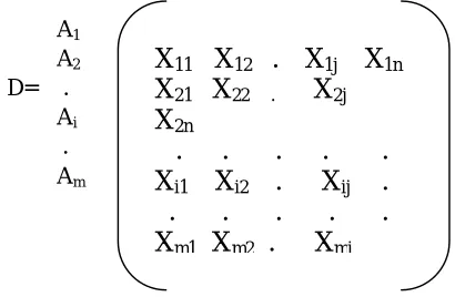
This step involves the development of matrix format. The row of this matrix is allocated to one alternative and each column to one attribute. The decision making matrix can be expressed as:

A1

A2

D= . Ai

. Am

1) Step 1: Construct normalized decision matrix.

2) Step2.Calculate the weighted normalized decision matrix v = [vij] . The weighted normalized value vij is calculated as vij = (wj)*(Rij) i=1,2……m,j=1,2,… n where wj is the weight of the jth attribute and

3) Step 3. Determine the positive ideal solution (PIS) V+ and negative ideal solution (NIS) V .

V+ = ,i=1,2…m}={V1+,V2+……Vn+}

V- = , i=1, 2…m} = {V1-, V2-……Vn-} Where J is a set of benefit attributes and J’ is a set of cost attributes.

4) Step 4. Calculate the separation measures, using the n dimensional Euclidean distance.

The separation of each alternative from the positive ideal solution i=I, 2….m

The separation of each alternative from the negative ideal solution

Calculate the relative closeness to the ideal solution

Ci= 0≤Ci≤1

Rank the alternatives with respect to Ci in descending order. By using experimental data decision matrix is designed.

TABLE SEPARATION VALUE AND IDEAL SOLUTION

V+MRR 0.018969

V-MRR 0.000825

V+RA 0.006378

V-RA 0.01972

X

X

. X

X

X

X

X

X

. . . . .

X

X

. X

.

VI. RESULTSANDDISCUSSION

According to Taguchi philosophy the use of loss function to measure the deviation between the experimental value and the desired value which is further transformed into signal-to-noise ratio (S/N). Basically, there are three types of categories in the evaluation of signal-to-noise ratio i.e.

Lower-the-better (LB), higher-the-better (HB) and nominal- the-better (NB) [20]. The objective of paper is to optimize the process parameter for MRR, and surface roughness (Ra). And for finding MRR higher the better has been taken to calculate the signal to noice ratio .and lower-the-better characteristic has been taken to calculate the other response parameter.

The optimal parameters were chosen based on higher S/N ratio as signal represents desirable value and noise represents undesirable value. Next, statistical analysis of variance (ANOVA) was conducted to study the significance of process parameters on responses based on their P-value and F-value at 95% confidence level.

200 150 100 2.2 2.0 1.8 1.6 1.4 1.2 0.20 0.15

0.10 0.3 0.6 0.9

A M e a n o f M e a n s B C

Main Effects Plot for Means Data Means 200 150 100 -2 -3 -4 -5 -6 -7 0.20 0.15

0.10 0.3 0.6 0.9

A M e a n o f S N r a ti o s B C

Main Effects Plot for SN ratios Data Means

Signal-to-noise: Smaller is better

Figure 6.1 main effect plot (Ra) for mean Fig 6.2 main effect plot for S/N ratio

From the above figure 6.1 we can see that as cutting speed increases from 100 to 150 m/min there is linearly decreases in surface roughness and it follows the reverse trend up to cutting speed value of 200m/min. According to main effect plots, average surface roughness is the lowest at levels speed 2, feed 1, DOC 3.

In the above figure 6.2 the s/n ratio of the surface roughness for corresponding parameter like speed, feed and DOC are most favorable at the point at A2, B1 and C3. So with the help of s/n ration graph and mean graph conclude that for minimum surface roughness the velocity should be average and feed should be minimum.

200 150 100 11 10 9 8 7 6 5 4 3 0.20 0.15

0.10 0.3 0.6 0.9

A M e an o f M e a n s B C

Main Effects Plot for Means

Data Means 200 150 100 20 18 16 14 12 10 0.20 0.15

0.10 0.3 0.6 0.9

A M e a n o f S N r a ti o s B C

Main Effects Plot for SN ratios

Data Means

Signal-to-noise: Larger is better

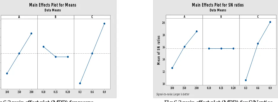
Fig 6.3 main effect plot (MRR) for means Fig 6.3 main effect plot (MRR) for S/N ratios

B A 0.20 0.18 0.16 0.14 0.12 0.10 200 180 160 140 120 100 > – – – – – < 1.2 1.2 1.4 1.4 1.6 1.6 1.8 1.8 2.0 2.0 2.2 2.2 Ra

Contour Plot of Ra vs A, B

B A 0.20 0.18 0.16 0.14 0.12 0.10 200 180 160 140 120 100 > – – – – – < 4 4 6 6 8 8 10 10 12 12 14 14 MRR

Contour Plot of MRR vs A, B

Figure 6.4 contour Plot of Ra Vs A, B Figure 6.5 contour Plot of MRR Vs A, B

C A 0.9 0.8 0.7 0.6 0.5 0.4 0.3 200 180 160 140 120 100 > – – – – – < 1.2 1.2 1.4 1.4 1.6 1.6 1.8 1.8 2.0 2 .0 2.2 2.2 Ra

Contour Plot of Ra vs A, C

Figure 6.6 contours Plot of Ra Vs A, C

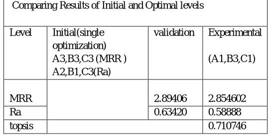
A. Conformation Or Validation Test

The confirming test is very important in verifying the improvement of machining performance characteristics in the analysis of optimization. In this study,

Comparing Results of Initial and Optimal levels

Level Initial(single optimization) A3,B3,C3 (MRR ) A2,B1,C3(Ra)

validation Experimental

(A1,B3,C1)

MRR

2.89406 2.854602

Ra 0.63420 0.58888

topsis 0.710746

B. Confirmation Test

VII. CONCLUSION

By using TOPSIS experimental data decision matrix has been developed. The weighted normalized decision matrix is constructed. In this approach, the distance values of each alternative from ideal and anti-ideal solutions are calculated by using concept of ranking method finally, the closeness coefficients are defined to attain the ranking order of all alternative combination of different machining parameter. And optimum value of among all combination is speed 100 m/min, feed 0.2 mm/rev and depth of cut is 0.3mm.

REFERENCES

[1] 1.P. J. Ross, Taguchi techniques for quality engineering, McGraw-Hill, New York, 1996.

[2] 2.G.Taguchi, Introduction to quality engineering, Asian productivity organization, Tokyo, 1990.

[3] 3.J. L. Lin, K. S. Wang, B. H. Yan, and Y. S. Tarng, Journal of Materials Processing Technology.,vol. 102, pp. 48

[4] 4. Ashok Kumar Sahoo ,Swastik Pradhan, Journal of measurement(2013)

[5] 5. Carmita Camposeco-Negrete Journal of Cleaner Production(2013) Optimization of cutting parameters for minimizing energy consumption in turning of

AISI 6061 T6 using Taguchi methodology and ANOVA

[6] 6. Debabrata Mandal, Surjya K. Pal ∗, Partha Saha Journal of Materials Processing Technology 186 (2007)

[7] 7. C.L. Lin, J.L. Lin, T.C. Ko, Optimisation of the EDM process based on the

[8] orthogonal array with fuzzy logic and grey relational analysis method, Int.

[9] J. Adv. Manuf. Technol. 19 (2002) 271–27

[10] 8. P. Asokan & R. Ravi Kumar & R. Jeyapaul & M. Santhi Development of multi-objective optimization models

[11] for electrochemical machining process(2008)

[12] 9. Rajesh Kumar Bhushan*Journal of Cleaner Production (2013)

[13] 10. Issam Hanafi a,*, Abdellatif Khamlichi a,1, Francisco Mata Cabrera b,2, Emiliano Almansa b,2,Abdallah Jabbouri c,3 Journal of Cleaner

Production(2012)

[14] 11. Ashvin J. Makadia J.I. Nanavati the Journal of measurement(2013),1Optimisation of machining parameters for turning operations based on response

surface methodology

[15] 12. Hae-Sung Yoon a, Jong-Seol Moon a, Minh-Quan Pham a, Gyu-Bong Lee b,