Parallel Preconditioners for Stokes Flow
A. Wildeman
NACM
Applied Mathematics
University of Twente
Master’s Thesis
Parallel Preconditioners
for Stokes Flow
Author:
Albert Wildeman
Supervisors:
Prof.dr.ir. J.J.W. van der Vegt Dr. M.A. Bochev
Contents
1 Introduction 4
2 Amphi3D 6
2.1 Diffuse Interface Method . . . 6
2.2 Finite Element Formulation . . . 8
2.3 Adaptive Mesh Generation . . . 10
2.4 Parallelization of Amphi3D . . . 10
3 Parallel Algebraic Preconditioning 12 3.1 Incomplete decomposition . . . 15
3.2 Sparse approximate inverses . . . 17
3.2.1 Frobenius norm minimization . . . 17
3.2.2 Biconjugation . . . 18
3.3 Algebraic multigrid . . . 19
4 Stokes flow test case 21 4.1 Description of algorithm . . . 21
4.1.1 The Governing Equations and Boundary Conditions . . . . 21
4.1.2 Weak Formulation and discretization . . . 23
4.2 Solution of the linear systems . . . 25
4.2.1 Properties of the linear systems . . . 26
4.2.2 Reordering . . . 27
4.2.3 Symmetric diagonal scaling . . . 27
4.2.4 Use of BiCGStab(`) . . . 28
4.3 Parallel Preconditioners . . . 28
4.3.1 Block Jacobi . . . 28
4.3.2 PILUT . . . 29
5 Software issues 35
5.1 Reordering and scaling . . . 35
5.2 Larger grid sizes . . . 36
5.3 HYPRE . . . 36
6 Results 38 7 Conclusions 43 Appendix: A Derivation of the weak formulations 45 A.1 Amphi3D . . . 45
A.1.1 The momentum equation . . . 45
A.1.2 The continuity equation . . . 47
A.1.3 The stress equation . . . 47
A.1.4 The Cahn-Hilliard equation . . . 47
A.2 Stokes flow . . . 49
A.2.1 The momentum equation . . . 49
A.2.2 The penalized continuity equation . . . 49
B The integration of PETSc in Amphi3D 50 B.1 Initialization, input and output . . . 50
B.2 PETSc datastructures . . . 51
B.3 Matrix memory preallocation . . . 52
Summary
Chapter 1
Introduction
Amphi (Adaptive Meshing for φ, the phase-field parameter) is a numerical algo-rithm for the solution of two-phase complex fluid flows. The use of a phase field parameter to distinguish between the two phases is its key feature, but the ex-tremely fine mesh this requires for adequate resolution of the thin interfacial layer results in very large meshes, despite the use of adaptive meshing. As this require-ment is even more pronounced in 3D, only very small 3D problems can be modeled with sufficient accuracy at reasonable computation times. In order to enable its application in the exploration of new and physically relevant flow problems, a parallel version of the algorithm was recently implemented. The approach was to leave the sequential code largely intact, and handle only the solution of the linear systems, which accounts for the bulk of the overall computational load, in parallel. The set-up of the linear systems and preconditioners, as well as the application of Krylov iterative solvers, is done through PETSc, a Portable, Extensible Toolkit for Scientific Computation [4]. This is essentially a library of functions, such as parallel linear and nonlinear solvers, built on top of MPI, the Message Passing Interface.
Several surveys [13, 57, 106] of parallel preconditioners have been published, but publications featuring direct numerical comparison of multiple parallel pre-conditioners are less common. Two papers by Ma [84, 85] approach the nature of this report, but the lack of the Stokes flow case and, much more imporantly, the dominant role of the reordering schemes associated with regular grids prevent a meaningful comparison to these papers.
Chapter 2
Amphi3D
In a system of two immiscible fluids, the interface plays a central role in the fluid dynamics and rheology. The mathematics of such a system is generally compli-cated by the movement of the interface, even more so when break-up or coalescence have to be accounted for. Two general strategies have emerged to encompass the evolution of the interface; interface tracking and phase-field methods. The former is a Lagrangian approach which directly tracks the interface with a fixed set of gridpoints, a process which becomes problematic when break-up or coalescence occur. In contrast, these phenomena are incorporated naturally in a phase-field framework such as Amphi, where the morphology is described by a continuous phase-field parameter. Furthermore, a diffuse interface is more physical in the sense that real interfaces have a finite thickness, or mixing region. The interfacial thickness used in simulations is, however, unphysically large for numerical rea-sons, but it leads to an energy-based variational formalism which allows a natural inclusion of complex fluid rheologies, on the condition that they can be described by a free energy.
Amphi3D can essentially be split into three different parts: the diffuse interface method, its finite element formulation and the adaptive meshing scheme.
2.1
Diffuse Interface Method
mixing energy. The phase-field variableφis defined to indicate the concentrations of the Newtonian and the Oldroyd-B fluid with (1+φ)/2 and (1−φ)/2, respectively. The mixing energy takes the Ginzburg-Landau form [24]:
fmix(φ,∇φ) =
1 2λ|∇φ|
2+ λ
42(φ
2−1)2 (2.1)
whereλrepresents the mixing energy density andis the capillary width, propor-tional to the width of the diffuse interface. The surface tension can be extracted from the ratioλ/ as→0 [69, 131]:
σ = 2
√
2 3
λ
(2.2)
Through Young’s equation,σcosθS=σw2−σw1, the fluid-solid interfacial tensions
σw1 and σw2 for the two fluids determine the static contact angleθS. The
diffuse-interface wall energy thus becomes [35, 70, 132]
fw(φ) =−σcosθS
φ(3−φ2)
4 +
σw1+σw2
2 . (2.3)
The evolution ofφ is governed by the Cahn-Hilliard equation:
∂φ
∂t +v· ∇φ=γ∇
2G (2.4)
where the chemical potential reads
G= δ
R
fmixdΩ
δφ =λ
−∇2φ+φ(φ
2−1)
2
(2.5)
and γ is the mobility [131].
The elastic energy of the Oldroyd-B fluid is described in [24]:
fd=
1 +φ
2
Z
R3
kTln Ψ + 1
2HQ·Q
ΨdQ (2.6) withndenoting the number density of the dumbbells, kthe Boltzmann constant,
T the temperature, H the elastic spring constant, Ψ(Q) the configuration distri-bution and Q is the vector connecting both ends of the spring.
The stress tensor τd is obtained by applying a variational procedure to the
total free energy, and satisfies the Maxwell equation [131, 133]:
where λH = ζ/(4H) is the relaxation time, the subscript(1) denotes the upper
convected derivative, ζ is the friction coefficient between the dumbbell beads and the suspending solvent and µp =nkT λH is the polymer viscosity. Upon addition
of the viscous stresses, the total stress tensor without the contribution of the mixing energy becomes
τ =
1−φ
2 µn+ 1 +φ
2 µs
[∇v+ (∇v)T] +1 +φ
2 τd (2.8)
with µn and µs denoting the viscosities of the Newtonian component and the
Newtonian solvent, respectively. With this stress tensor, the equations of motion can be written as
ρ
∂v
∂t +v· ∇v
=∇ ·(−pI+τ) +G∇φ+ρg (2.9)
∇ ·v = 0 (2.10)
where ρ = 1+φ2 ρn+ 1−φ2 ρs with ρn and ρs the densities of the Newtonian and
Oldroyd-B fluids, respectively, and similarlyµ= 1+φ2 µs+1−φ2 µn.
Furthermore, g is the gravitational acceleration and G∇φ is the interfacial stress, the diffuse-interface representation of the inertial forces on both fluids [131].
The boundary conditions come to
v−vw = 0 (2.11)
on the solid wall boundary (∂Ω)u, with vw denoting the velocity of the wall, and
n· ∇G= 0 (2.12)
λn· ∇φ+fw0 (φ) = 0 (2.13) on the entire boundary∂Ω, withndenoting the unit normal to the boundary. The no-slip condition, (2.11), leaves Cahn-Hilliard diffusion as the sole source of contact line motion. Mass conservation of both fluids follows from (2.12), which ensures zero flux through the solid wall and mass conservation of each fluid. Finally, (2.13) is the natural boundary condition from the variation of the wall energy fw, and
the left-hand side represents the surface chemical potential. Thus, this condition entails that the fluid layer is always at equilibrium with the solid substrate.
2.2
Finite Element Formulation
element and continuous across element boundaries, do not accomodate the repre-sentation of spatial derivates of order higher than two. To circumvent this issue, the Cahn-Hilliard equation (2.4) is decomposed into two second-order equations:
∂φ
∂t +v· ∇φ= γλ
2∆(ψ+sφ) (2.14)
ψ=−2∆φ+ (φ2−1−s)φ (2.15) The parameterswas introduced to enhance stability of the numerical method and in all applications to date [133, 135], s = 0.5 has been adequate. A convenient side effect of this value is that it reduces the chemical potential toG=λ(ψ+sφ). The weak solution sought is (v, p, τd, φ, ψ) ∈ U × P × T × S × S, where for
3D flows, the solution spaces satisfy U ∈ H1(Ω)3, P ∈ L2(Ω), T ∈ L2(Ω)6, and S ∈H1(Ω). The weak form of the governing equations with basis functions (˜v,p,˜ τ ,˜ φ,˜ ψ˜), is derived in appendix A.1:
Z Ω ρ ∂v
∂t +v· ∇v−g
−G∇φ
·v˜+ (−pI +τ) :∇v˜
dΩ = 0 (2.16)
Z
Ω
(∇ ·v)˜p dΩ = 0 (2.17)
Z
Ω
τd+λHτd(1)−µp
∇v+ (∇v)T : ˜τ dΩ = 0 (2.18)
Z
Ω
∂φ
∂t +v· ∇φ
˜
φ+γλ
2 ∇(ψ+sφ)· ∇φ˜
dΩ = 0 (2.19)
Z
Ω
n
ψ−(φ2−1−s)φψ˜−2∇φ· ∇ψ˜
o
dΩ−
Z
∂Ω
2 λf
0
w(φ) ˜ψ dS= 0 (2.20)
The associated boundary conditions take the following form:
v−vw = 0 on (∂Ω)u (2.21)
(−pI+τ)·n= 0 on (∂Ω)τ (2.22)
τd−τin = 0 on (∂Ω)in (2.23) ∇φ·n+fw0(φ)/λ= 0 on ∂Ω (2.24)
∇(ψ+sφ)·n= 0 on ∂Ω (2.25) where∂Ω = (∂Ω)uS(∂Ω)τ, (∂Ω)uT(∂Ω)τ =∅and (∂Ω)in is the inflow boundary.
Note that the natural boundary condition (2.24) was used in the derivation of (2.20).
tetrahedral mesh. Upon spatial discretization of (2.16-2.20) the nonlinear algebraic system is cast in the form
Λ·
∂U
∂t
n+1
+F Un+1= 0 (2.26) whereU is the solution vector,Λa diagonal matrix with only zeros and ones on the diagonal, depending on the appearance of the corresponding component ofU in a time derivative. All other terms are collected in F. A fully implicit second-order scheme is applied to discretize the time derivative, upon which (2.26) is solved with an inexact Newton method using backtracking for improved convergence and stability, as described in [53]. The common technique of using the Jacobian matrix within the Newton method for a number of iterations rather than updating it for every iteration is employed to reduce the computational effort.
2.3
Adaptive Mesh Generation
To achieve fine resolution of the interface with realistic mesh sizes, Amphi employs the GRUMMP (Generation and Refinement of Unstructured, Mixed-Element Meshes in Parallel) adaptive meshing scheme [59]. Rather than tracking the interface, the mesh is principally static but coarsened and refined as the interface moves through the domain. As GRUMMP takes a scalar field LS to control the mesh size using
Delaunay refinement, it is natural to use the gradient of the phase-field variable
φ to determine this scalar field. Specifically, the form used for the 2D algorithm is left unaltered in the 3D version:
LS(x, y, z) =
1
|∇φ| √
2 C +
1 h∞
, (2.27)
where C is a parameter controlling the resolution of the interface and h∞ is the
mesh size in the bulk. At the interface, the thickness of which scales with ,LS
becomes h1 ≈C·. So far, simulations have been run with values forC ranging
from 0.5 to 1, and proper mesh resolution was achieved for C = h1 ≤ . As
the interface has a thickness of approximately 7.5, it will be covered by roughly 10 gridpoints. Furthermore, h∞ is actually split into h2 and h3 to allow different
mesh densities in the bulk of each fluid, and there is another parameter controlling the sensitivity of the intended mesh density to the distance from the interface.
2.4
Parallelization of Amphi3D
it is for this reason that a parallel version of the code was designed. To this end, it was decided to employ PETSc, a Portable, Extensible Toolkit for Scientific Computation [4].
The PETSc manual states quite clearly that parallelization through the use PETSc should not take the form where PETSc is called to solve a linear system in parallel in an otherwise sequential code [4], as matrix assembly will take too much time in this scenario. Instead, PETSc, and therefore parallelization, should be involved at least in the matrix assembly.
In brief, the Amphi3D algorithm combines a finite-element flow solver and the GRUMMP adaptive meshing scheme. Combined with a Crank-Nicholson temporal discretization, this leads to a nonlinear system which is solved by an inexact Newton method. Importantly, the nonlinear system is not explicitly available in the code, and it would take considerable effort to write a function representing this nonlinear system. However, such a function is prerequisite to invocation of a PETSc nonlinear solver. Therefore, PETSc has to be involved at a lower level, that is within the inexact Newton method. Each Newton iteration consists of the assembly of a system matrix and the solution of the corresponding linear system, which, as mentioned earlier, is also the lowest level at which PETSc parallelization can be efficient. This motivated the decision to use PETSc, that is to parallelize, at the level of matrix assembly and solution of the linear system within each Newton iteration. Details of the incorporation of PETSc in the parallel code are collected in appendix B.
Chapter 3
Parallel Algebraic
Preconditioning
The convergence rate of Krylov subspace methods is depends strongly on the properties of the linear system it is applied to. In particular, performance improves as the eigenvalues are more tightly clustered and often as they are closer to unity. Preconditioning is the process of transforming the original linear system Ax= b
to an equivalent one, with favorable properties facilitating the convergence of a Krylov subspace method applied to solve the system.
Preconditioning is widely regarded as the most important part in the design of an efficient iterative solution strategy [57, 73] as well as the most difficult to parallelize [13, 124]. In fact, solution of many problems only becomes feasible upon its application. The importance of preconditioning was sharply indicated by Trefethen and Bau in [119]:
In ending this book with the subject of preconditioners, we find ourselves at the philosophical center of the scientific computing of the future. (...) Nothing will be more central to computational science in the next century than the art of transforming a problem that appears intractable into another whose solution can be approximated rapidly. For Krylov subspace matrix iterations, this is preconditioning.
Preconditioning is usually effected by a matrix called the preconditioner. This nonsingular matrix,M, can be applied to the original linear system to transform it into
M−1Ax=M−1b (3.1)
to those of the original linear system. When M−1 is explicitly known, such as for polynomial or sparse approximate inverse preconditioners, M itself is never constructed. On the other hand, M−1 is usually never explicitly formed if M is given. System (3.1) is the result of left preconditioning, but right preconditioning, resulting in
AM−1y=b, x=M−1y (3.2) and split preconditioning,
M1−1AM2−1y=M1−1b, x=M2−1y (3.3) are also commmonly used, the latter intended primarily to preserve symmetry or near-symmetry when it is present in the orginal system. Note that in (3.3), the preconditioner isM =M1M2. Which of these types of preconditioning is most
ef-fective depends primarily on the Krylov subspace method used and the properties of the system matrix. GMRES, for example, tends to favor right precondition-ing [13]. The system matrices of the transformed systems, M−1A, AM−1 and
M1−1AM2−1 are similar and therefore have the same spectrum. As a result, the convergence of the CG method in exact arithmetic is identical for each system if both A and M are symmetric positive definite. On the other hand, the behavior of GMRES and other Krylov subspace methods can depend strongly on left or right positioning of the same preconditioner [123]. A striking example of such dependence can be found on p.66 of [79].
Importantly, the system matrices of the transformed systems are never explic-itly calculated. Rather, matrix-vector products and the solution of linear systems of the form M z =b suffice, and in the case where M−1 is known explicitly only matrix-vector products are required.
The choice for a particular preconditioner is necessarily a compromise between three base criteria [13, 122]:
• The Krylov subspace method should converge rapidly for the preconditioned system
• The preconditioner should be inexpensive to construct
• The operator M−1 should be inexpensive to apply
subspace methods and preconditioners to begin with. Therefore, the second and third property voice the concern for excessive overhead before the iterative pro-cess can commence and the overhead in each iteration, respectively. Naturally, the balance between these issues is aimed at minimization of the overall computing time. Although most preconditioning techniques are aimed at the approximation
M−1 ≈ A−1, or equivalently, at bringing all eigenvalues of the preconditioned linear systems to unity, interesting exceptions exist; see [92] for an example. Situ-ations where a series of linear systems with identical system matrix and different right-hand sides has to be solved constitute a strong shift in this balance, as the expense of preconditioner construction can be amortized by its application to re-peated solves. This tends to be the case when the linear systems arise from some variant of Newton’s method.
For parallel preconditioners, great care must be taken to limit the amount of cross-process communication, both in its construction and application. The latter suggests that the preconditioner should be as close to block diagonal as possible, with each block corresponding to the unknowns on one processor.
A first classification of preconditioners can be made in terms of generality. Many applications involving PDEs employ preconditioners which are near-optimal for a very narrow set of problems. These are generally based on complete knowl-edge of the underlying problem; not only in terms of its governing equations, but also with respect to the geometry, the boundary conditions and the details of the discretization. Preconditioners based on a simplified version of the governing equations or lower order discretization belong to this class. Multigrid precondi-tioners are often employed in this manner [91], but can also be fully algebraic [115].
The primary drawbacks of the problem-specific approach is that it requires the solver developer to have a complete understanding of the problem, and that the often considerable effort in designing the preconditioner can be applied only to a very narrow range of problems as a result of the sensitivity of the effective-ness of these preconditioners to the details of the problem. These arguments have motivated the enduring quest for widely applicable, purely algebraic precondition-ing methods which use nothprecondition-ing but the system matrix. Although this approach cannot be expected to rival the quality of application-specific preconditioners, they can achieve reasonable efficiency and offer greater flexibility when details of the underlying problems are altered. They are particularly well-suited for prob-lems with unstructured meshes, and often can be fine-tuned to fit the underlying problem, thus blurring the distinction between general and application-specific preconditioners. Furthermore, specific preconditioners are generally based on ex-isting algebraic methods, as exemplified by [125].
the focus of this chapter lies with the three primary classes of algebraic pre-conditioners: incomplete factorization, sparse appoximate inverses and algebraic multigrid.
3.1
Incomplete decomposition
Incomplete decomposition preconditioning techniques are among the oldest and most frequently used, in both sequential en parallel settings. Guassian elimi-nation generally generates considerable fill-in when decomposing a sparse matrix. Sparsity-preserving pivoting techniques have been developed, but for many classes of linear systems, the resulting sparse direct method tends to be far too costly, primarily in terms of memory, to execute for large sparse matrices. Incomplete decomposition is based on the notion of dropping part of the fill-in which is in some sense unimportant to the quality of the decomposition; creating a precondi-tioner M = ˜LU˜, with ˜L and ˜U denoting the approximate, or incomplete, factors ofA, respectively. The primary distinction between variants of incomplete factor-ization techniques concerns the criteria upon which fill entries are dropped from the factors.
For symmetric matrices, incomplete Cholesky factorization or IC is used, but this chapter will focus on incomplete LU factorization, ILU, as the matrices of both Amphi3D and the Stokes flow test case at hand are nonsymmetric. A family of ILU preconditioners known as ILU(k), was introduced in [64, 128] and allows fill-in up to levelk. A thorough exposition on fill levels is available in [13]. Another popular ILU variant is ILU(τ), which simply drops any fill entries whose absolute value is smaller than the threshold τ. The difficulty of predicting the amount of fill and associated memory requirement is a drawback of both ILU(l) and ILU(τ), and motivated the development of the dual threshold ILUT(τ,p) algorithm [101], which employs a drop tolerance like ILU(τ) but adds the requirement that onlyp
fill-in entries are kept in each row of the incomplete LU factors.
In principle, increasing fill-in improves the convergence rate of the Krylov solver, but there have been observations [49] of non-monotonic improvement of the convergence with increasing fill-in in the preconditioner.
With the introduction of parallel computation, the subject of parallel precondi-tioning immediately arose, as the prevalent ILU techniques are not readily suited for such application by the inherent sequential nature of Gaussian elimination. Furthermore, the forward and backward solves that have to be conducted at each iteration are highly sequential.
preconditioners deteriorates rapidly as the number of processors increases. No-fill ILU can also be parallelized to fair extent through the application of graph coloring techniques, but it too is generally insufficient to achieve a satisfac-tory rate of convergence in the Krylov subspace solver. Better convergence can be achieved by allowing some fill-in, but this drastically increases cross-process communication.
Another approach to the parallelization of ILU preconditioning is to embed the factorization in domain decomposition. The Additive Schwarz method [113], or ASM, constructs a preconditioner by dividing the problem domain into a number of possibly overlapping subdomains and subsequently combining the subdomain preconditioners. The communication between the subdomains through the over-lap can be realized in any of a number of ways [50], or the overover-lap can be set to zero; reducing the preconditioner to Block Jacobi. Note that although incom-plete decomposition techniques are prevalent, Additive Schwarz methods can use any preconditioner for its subdomains. Regardless of the internal preconditioner, however, the convergence of the iterative solver is often poor as a consequence of the relatively crude coupling of the subdomains. One approach to reinforce global coupling is the addition of an extra layer on top of Additive Schwarz in the form of a coarse-grid correction, resulting in a multilevel method [113].
Techniques where reordering is applied with the goal of assigning numbers that are not too far apart to neighbouring grid points or unknowns were first introduced in [52, 121]. Recent versions of this idea can be found in [110, 1, 90, 67, 68] and have been shown to be quite efficient for select problems. The algorithm sug-gested in [68] is scalable, which means that the work involved in constructing the preconditioner remains constant when the problem size and number of processors are increased with equal factors. The algorithm divides the factorization problem into a number of non-overlapping subproblems of roughly equal size which can be solved in parallel. Each subproblem is divided into edge elements and interior elements; first, only the interior of each subdomain is factored, thereafter rows corresponding to boundary elements are factored. The latter step requires cross-process communication, the limitation of which depends strongly on the possibility of a clean cut, or relatively small total edge length, between the subdomains.
3.2
Sparse approximate inverses
The central idea of sparse approximate inverse preconditioning is that the pre-conditioner is an explicitly computed approximation to the inverse of the system matrix A;M−1≈A−1. Importantly, the construction of such a preconditioner is fully parallel when the approximation is executed on suitable criteria. Further-more, there is no inherent risk of breakdown as for ILU and the approach is very robust. Even though the inverse of a sparse matrix is generally dense, and it can even be proven that irreducible sparse matrices have structurally dense inverses [51], many entries of the inverse of a sparse matrix tend to be small in absolute value; creating the opportunity for a close sparse approximation.
Two basic types of approximate sparse inverse preconditioning exist; one where
M is a single matrix and one where it is the product of any number of matrices. The latter approach is commonly referred to as factored sparse approximate in-verses and is related to the LU factorization ofA:
M =MLMU, whereML≈L and MU ≈U (3.4)
assumingAhas an LU decomposition. For both the factored and unfactored cases, two manners of approximation have emerged: Frobenius norm minimization and incomplete (bi-)conjugation.
3.2.1 Frobenius norm minimization
The oldest form of sparse approximate inverses dates back to the seventies [11, 58, 12] and employs the Frobenius norm to compute an approximate inverseM−1
[62]:
||AM−1−I||2F =
n
X
k=1
||(AM−1−I)ek||22 (3.5)
Crucially, minimizing in the Frobenius norm is completely parallel as it can be split into
min(M−1)
k ||A(M
−1
)k−ek||2, k= 1, ..., n (3.6)
elements which contribute most to the minimization (3.6), up to the point where a maximum number of nonzeros for the row has been reached or the row is close enough to the corresponding row in the inverse of A to meet a certain tolerance. Although all the algorithms within the general framework discussed in this section are sparse approximate inverse methods, the abbreviation SPAI is associated with [62] specifically. This algorithm has proven to be the most successful of its kind and can result in very good convergence of the Krylov solver, but parallelization is far from trivial, as illustrated by the parallel implementations [9, 8], and construction of the preconditioner is very expensive [20].
The latter issue formed the motivation for the introduction of the Minimal Residual method [42], which replaces the exact minimization of (3.6) by a few iterations of a minimal residual method. An added benefit of this approach is that, contrary to SPAI, there is no prescribed initial sparsity pattern required. On the other hand, this technique was observed to be less robust [20]. A yet different class of algorithms has been developed where an effective sparsity pattern is automatically generated, the most notable of which is ParaSAILS, the subject of Section (4.3.3).
A factored, Frobenius-norm minimization approximate inverse preconditioner, FSAI or Factored sparse approximate inverse, was introduced in [75]. It has performed very well forsymetric positive definite (SPD) matrices [14, 76]; retaining the SPD property for the preconditioner of such matrices and therefore enabling the use of the conjugate gradient Krylov method. The preconditioner, M =
MLMLT, is conceptually constructed by a sparse approximation to the Cholesky
factor of the system matrix; however, it is computed using only the values A
and the Cholesky factor is never computed. Details involved with the parallel implementation of FSAI can be found in [23, 41, 46, 55]. Notwithstanding the symmetric roots of FSAI, extension to general sparse matrices has been realized. However, its application to nonsymmetric matrices has proven both unreliable and ineffective [15], with AINV (Approximate inverse), which will be described shortly, consistently achieving superior efficiency.
3.2.2 Biconjugation
independently by [14] and [72].
Although the application of the preconditioner is easily parallelized, its con-struction is, not unlike ILU, inherently sequential. The rather crude solution of constructing the preconditioner in a sequential manner and subsequently broad-casting it to all other processes as in [22] is simple, but time-consuming and possible only when the problem size is sufficiently small for this to approach to be viable in terms of its memory requirement. Parallel construction of this pre-conditioner has been achieved through graph partioning [16, 21] and compared favorably to a number of multigrid methods [13, 114]. Further developments of AINV have been presented in [29, 30, 31, 22, 23, 26, 86, 87, 88, 60, 97].
3.3
Algebraic multigrid
Algebraic multigrid methods, or AMG [99], are best understood as a generaliza-tion of geometric multigrid methods, which in turn are an extension of geometric two-grid methods. The latter is based on the introduction of a coarse grid in addition to the grid with the resolution of the desired solution. The solution strategy then consists of alternating reduction of the error on the fine grid, known as smoothing, and reduction of the error on the reduced grid, known as coarse grid correction. In algebraic multigrid, the coarse and fine grid distinction is no longer based on the physical domain of the problem, but extracted from the system matrix. As such, there is no direct link between the algebraic multigrid approach and Krylov subspace methods or preconditioners. However, the two ap-proaches, though conceptually and historically distinct, have been combined in various froms; including the use of multigrid solvers within block preconditioners for Krylov solvers [127] and the application of preconditioners designed for Krylov solvers as smoothers for multigrid. In the latter category, incomplete factorization has been applied [129], but recent work in this area has focused on the applica-tion of sparse approximate inverses in this manner [33, 32, 117, 116]. Conversely, the difficulty of scalability of preconditioners for Krylov solvers has motivated the quest for variants which include elements of the multigrid approach. Although no particular algorithm has surfaced as the fastest or most robust, a lot of work has been done on multigrid variants of incomplete factorization preconditioners [100, 107, 108, 98, 5, 7, 6, 28, 48, 80, 94, 95, 105, 120, 134] and sparse approximate inverse preconditioners [25, 87, 88, 93].
Although parallelization of algebraic coarsening has proven troublesome, par-allel AMG is a young [43] but active field of research [77, 63, 65, 89, 130]. However, little has been achieved in their application to indefinite matrices, or systems aris-ing from three dimensional partial differential equations.
Chapter 4
Stokes flow test case
As alluded to in the introduction and illustrated in the previous chapter, the op-tions for parallel preconditioning of a complex system of equaop-tions in algorithms like Amphi3D are plenty. However, finding an effective preconditioner for Am-phi3D has proven very difficult. Rather than through trial and error, this project approaches the situation by comparing parallel preconditioners on the much re-duced problem of Stokes flow, anticipating that evaluation of preconditioner per-formance for this problem will provide a solid basis for a more structured, educated and hopefully more fruitful process of preconditioner selection. Instead of writing a new code, a third party Matlab code was selected to serve as the framework for the simulations and generate linear systems to serve as test cases for parallel pre-conditioners. This code,NS3D_FEM(Navier-Stokes 3D, finite element method)[27], does, however, use a different formulation of the problem. This chapter opens with a discussion of that algorithm, followed by a discussion of the details of the linear systems as well as the parallel preconditioners tested on these systems.
4.1
Description of algorithm
4.1.1 The Governing Equations and Boundary Conditions
The problem at hand is steady-state and does not include gravity, but is techni-cally a low Reynolds number Navier-Stokes flow rather than a pure Stokes flow. The starting point is comprised of the usual steady, incompressible Navier-Stokes equations with zero body force:
where ν is the kinematic viscosity, v is the velocity vector and p is the pressure. The test case describes flow around a sphere in a cylinder; the domain Ω used in these simulations is a cylinder around the z-axis with a radius of 2 and ranging from z=−2 toz= 7. The sphere is situated at the origin and has a radius of 12. The inflow boundary (∂Ω)in is situated atz=−2, the outflow boundary (∂Ω)out
atz= 7 and the no-slip boundary (∂Ω)wall is comprised of the wall of the cylinder
x2+y2 = 4 and the sphere at the origin, x2 +y2 +z2 = 1/2. The boundary conditions come to
v=
0,0,1−1
4 x
2+y2) T
on (∂Ω)in (4.3)
ν∂v
∂n+np= 0 on (∂Ω)out (4.4) v= 0 on (∂Ω)wall (4.5)
-2 -1 0 1 2 -2
-1 0 1 2 3 4 5 6 7
X Y
Z
z
y
Figure 4.1: A cross section of the domain along x = 0. The greyscale indicates velocity in the z-direction, with lighter shades corresponding to higher velocities.
4.1.2 Weak Formulation and discretization
Rather than a traditional weak formulation based directly on Equations (4.1) and (4.2), the algorithm of NS3D_FEM includes the addition of a penalty term to the continuity equation, restating the system of equations as
−ν∇2v+v· ∇v+∇p= 0 (4.6)
∇ ·v+
νp= 0 (4.7)
whereis the penalty parameter. Through the derivation of appendix A.2.1, this results in the weak formulation
Z
Ω
ν∇v:∇v˜+ (v· ∇v)·v˜−p∇ ·v˜dΩ = 0, (4.8)
Z
Ω
(∇ ·v+
νp)˜p dΩ = 0. (4.9)
The nonlinear term∇v·v˜ necessitates the use of a Newton method, as is the case in Amphi3D. This results in a series of iterates (vk, pk), k ∈ 1,2, ... converging,
in principle, to the solution of the weak formulation. The initial guess (v0, p0) in
the NS3D_FEM code satisfies the boundary conditions. Given the iterate (vk, pk),
the nonlinear residual (Rk, rk) associated with the momentum part of the weak
formulation reads:
Rk=
Z
Ω
−(vk· ∇vk)·v˜−ν∇vk:∇v˜+pk∇ ·v˜dΩ (4.10)
rk=
Z
Ω
−p˜(∇ ·vk+
νpk)dΩ (4.11)
With v = vk +δvk and p = pk+δpk the solution of the weak formulation, it
follows that
D(vk, δvk,v˜) +
Z
Ω
ν∇δvk:∇v˜−δpk∇ ·v˜dΩ =Rk(˜v) (4.12)
Z
Ω
˜
p(∇ ·δvk+
νδpk)dΩ =rk(˜v) (4.13)
where D(vk, δvk,v˜) is the difference in the nonlinear terms and can be expanded
as
D(vk, δvk,v˜) =
Z
Ω
(δvk+vk)· ∇(δvk+vk)·v˜−(vk· ∇vk)·v˜dΩ (4.14)
=
Z
Ω
Dropping the quadratic term, (4.15) is plugged back into (4.12), yielding the linear equations
Z
Ω
(δvk· ∇vk)·v˜+ (vk· ∇δvk)·v˜+ν∇δvk:∇v˜−δpk∇ ·v˜dΩ =Rk(˜v), (4.16)
Z
Ω
˜
p(∇ ·δvk+
νδpk)dΩ =rk(˜v). (4.17)
As usual for discretizations of the Navier-Stokes equation, mixed finite elements are used in the spatial discretization, and
vk+1,h = nu
X
j=1
vk+1j φj (4.18)
pk+1,h = nu+np
X
j=nu+1
pjk+1ψj (4.19)
whereφkis the set of vector-valued basis functions for the velocity, andψkthe set
of pressure basis fuctions. Furthermore nu holds the number of velocity degrees
of freedom, three times the total number of velocity nodes minus those associated with the Dirichlet boundary conditions, and np similarly denotes the number of
pressure degrees of freedom. Substituting (4.18, 4.19) into (4.16, 4.16) results in the system of linear equations
A BT
B C
[x] =
f g
(4.20)
where x= [v1
k+1, ...,v nu
k+1, p nu+1
k+1 , ..., p nu+np
k+1 ]T and
A(i, j) =
Z
Ω
{φj · ∇vk,h+vk,h· ∇φj} ·φi+ν∇φj :∇φidΩ (4.21)
B(i, j) =
Z
Ω
ψi∇ ·φjdΩ (4.22)
C(i, j) =
Z
Ω
νψiψjdΩ (4.23)
f(i) =
Z
Ω
− {vk,h· ∇vk,h} ·φi−ν∇vk,h:∇φi+pk,h∇ ·φidΩ (4.24)
g(i) =
Z
Ω
(∇ ·vk,h+
νpk,h)ψidΩ (4.25)
The element matrices and element vectors arising form this system are immediately apparent, as their form is identical to the matrix and right hand side, respectively, of (4.20). In fact, the only difference is that the domain of integration is the element rather than the entire domain, and that the integration is performed by a 5-point Gauss quadrature rule. The use of terahedral Taylor-Hood elements implies that the element matrices are 34×34 and the element vectors have length 34.
Taylor-Hood Elements
The Taylor-Hood element [118] was designed for mixed finite element problems, and the tetrahedral version features 10 nodes for the velocity components, one on each vertex and one in the center of each edge, and 4 pressure nodes, one on each vertex. In three dimensions, then, each element has 34 degrees of freedom in total.
where
A
(
u
)
is the advection and diffusion matrix,
B
is the pressure gradient
matrix,
B
Tis the divergence matrix and
I
is the identity matrix. The vectors
uand
p
form the velocity and the pressure discrete solution respectively. The mesh
size is denoted by
h. The scalar
α
is used for numerical convenience, which is
typically in the range 10
7-10
10(Zienkiewicz and Taylor, 1992) to account for the
lack of pivoting technique. In most cases, this system is large, sparse, non
symmetric (however for Stokes problem the matrix is symmetric) and ill
conditioned due to the zero entries that appear in the diagonal pressure
block-matrix.
a) b)
[image:27.595.219.355.326.387.2]c) d)
Figure 2 : Tetrahedral finite elements for fluid flow problems (velocity nodes left;
pressure nodes right): a) P2-P1 (Taylor-Hood); b) P2
+-P1 (Crouzeix-Raviart); c)
P1
+-P1 (MINI); d) P1
+-P0.
It is worth noting that the above discretized form may be modified to
account for time varying problems. An appropriate temporal discretization must
be used like unconditionally stable implicit first order Euler and second order
Crank-Nicholson and Gear schemes, or an explicit scheme associated with a time
step
Δtrestriction obeying the Courant-Friedrichs-Lewy (1928) condition:
1
≤ Δ
h t
u
(7)
Implicit schemes are usually preferred against explicit ones because they are more
robust. It must also be highlighted that mesh regularity is an important parameter
Heniche and Tanguy: Finite Element Modeling of Viscous Mixing: A Review
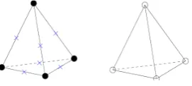
Figure 4.2: The 3D Taylor-Hood element. The dots and crosses in the left tetra-hedron represent the vertex and edge velocity nodes respectively; the circles in the right tetrahedron represent the presssure nodes.
4.2
Solution of the linear systems
For the preconditioner tests of this report, the first linear system arising in the Matlab code NS3D_FEM is written out as an ascii file and transferred to the Sara Huygens system. Subsequently, a Fortran code including the PETSc libraries is ran which reads the linear system, constructs the preconditioner and executes the Krylov solver. Although this is naturally not a viable option when running actual simulations, it does not affect the timings as the crucial steps, construction of the preconditioner and execution of the Krylov solver, would be identical in an all-Fortran code.
Sara Huygens is an IBM pSeries 575, clustered SMP (Symmetric Multipro-cessing) system consisting of 104 nodes, 16 dual core processors (IBM Power6, 4.7 GHz) per node, either 128 GByte or 256 GByte of memory per node. The smaller memory nodes are sufficient for these calculations. Huygens uses simultaneous
multithreading and recommends the usage of 64 MPI tasks per node. Use of this guideline means that jobs using more than 64 MPI tasks use multiple nodes, which implies the addition of slower, cross-nodal communication. Throughout the rest of this report, MPI tasks are referred to as processors for simplicity, although this is not strictly correct.
4.2.1 Properties of the linear systems
Calculations are executed for Reynolds numbers 1, 10 and 50. With the standard grid size, the problem has 4.1·104 elements and 5.9·104 nodes. By the use of Taylor-Hood elements, this results in 1.6·105velocity and 7.9·103pressure degrees of freedom, a square matrix of size 1.6·105 and 1.5·107 nonzeros. Grid sizes double and eight times the standard size with correspondingly larger matrix dimensions were also tested.
4.2.2 Reordering
The first operation performed on the linear systems is Reverse Cuthill-McKee reordering [61], which is aimed at the concentration of all nonzeros around the main diagonal. This is particularly important when solving the system in parallel as it reduces the number of connections between the variables across processors. The implementation ofNS3D_FEMinherently produces a matrix where the velocity components are already ordered in such a fashion, whereas the pressure nodes are segregated and unordered. The primary effect of the reordering, therefore, is the placement of the pressure degrees of freedom among the velocity degrees of freedom of the same nodes, as illustrated in Figure 4.3.
Figure 4.3: The sparsity structure of coefficient matrix before and after Reverse Cuthill-McKee reordering.
4.2.3 Symmetric diagonal scaling
After reordering of the linear system, symmetric diagonal scaling is applied to the linear system Ax=b:
D−1/2AD−1/2x˜=D−1/2b (4.27)
4.2.4 Use of BiCGStab(`)
In preliminary runs, BiCGStab(`) [111, 112], `= 2 surfaced as the fastest Krylov iterative solver for these matrices, and all further tests were conducted with this solver.
As the PETSc implementation of BiCGStab(`) only allows left preconditioning, all preconditioners tested are applied from the left. The iterations are said to have converged when the relative residual reaches below 1·10−6; in other words, when
||r||2 <1·10−6||b||2, wherer and bdenote the residual and the right hand side of
the linear system, respectively.
4.3
Parallel Preconditioners
As the symmetric diagonal scaling described in Section 4.2.3 is applied to the system matrices before all solves, they are reasonably conditioned even before a preconditioner is applied. This makes the solution of the system without further preconditioning feasible, and causes its inclusion in the comparisons to be more than a trivial point of reference. Apart from the unpreconditioned system, three preconditioners available through PETSc are tested. Block jacobi is included as it is the simplest of parallel preconditioners. PILUT has been included to represent the incomplete factorization class of preconditioners. This is a legacy code and no longer supported, but is the only preconditioner of this class available through PETSc outside Euclid, which was the first choice but foregone when it consistently crashed during preconditioner construction. PETSc offers access to two parallel approximate inverse preconditioners, SPAI and ParaSAILS (parallel sparse approximate inverse, least squares). The latter was selected as it is both the most efficient, according to a comparison in [40], and the most stable of the two.
4.3.1 Block Jacobi
4.3.2 PILUT
PILUT, introduced in [71], is a parallelization of the ILUT(m,t) algorithm of [101]. This warrants a consideration of the ILU(m,t) algorithm before the parallel aspects of PILUT are discussed.
The sequential algorithm: ILUT(m,t)
In order to limit the cost of both its construction and application, ILUT(m,t) em-ploys a dual dropping strategy. The general algorithm and the point of application for both dropping stages is illustrated in Figure 4.4.
1 for i = 1,...,n 2 w = a(i,*)
3 for k = 1,...,i-1
4 if w(k) != 0
5 w(k) = w(k)/a(k,k)
6 Apply first dropping rule to w(k)
7 if w(k) != 0
8 w = w - w(k)*u(k,*)
9 endif
10 endif
11 endfor
12 Apply second dropping rule to w 13 for j = 1,...,i-1
14 L(i,j) = w(j) 15 endfor
16 for j = 1,...,n 17 U(i,j) = w(j) 18 endfor
19 w = 0 20 endfor
Figure 4.4: The ILUT(m,t) algorithm
In this algorithm,wis a working row used to accumulate linear combinations of sparse rows in the elimination. The first dropping rule, applied in Line 6 of Figure 4.4, simply sets any element ofwto zero when it is smaller than the relative tolerance ti, the product of the parametert and the 2-norm of the ith row of A.
Line 12 features the second dropping rule, which initially one again drops all values below the relative tolerance ti, but additionally employs the second parameterm
mlargest elements of theUpart of the row. This results inm+ 1 elements per row of both Land Uas the diagonal elements are not subject to any dropping criteria. A discussion of proper data structures for efficient sequential implementation of this algorithm is featured in [101, 102].
The parallel algorithm: PILUT
The central idea of the PILUT algorithm of [71] is to separate those rows of the coefficient matrix which are internal to processor’s domain, that is have no connections to nonlocal rows, and those that do have such connections. The former category of rows is branded interior, whereas nodes, or rows, within the latter category are known as interface nodes.
The first step of the algorithm consists of each processor factoring its set of interior nodes, which is an entirely sequential process. Note that this is where the connection between PILUT and ILUT(m,t) resides; all the factorizations discussed in this Section are implemented as ILUT(m,t) factorizations. The values for the paramatersmandtused for the calculations of this report are the HYPRE default values of m = 20 and t = 1·10−4, respectively. In the second step, the interior nodes of all processors are eliminated from A, thus forming the reduced matrix
AI featuring only interface nodes. Factoring AI is subsequently executed by all processors cooperating, and it is in this phase that the communication resides, as well as the distinction between most parallel ILU algorithms.
PILUT performs the parallel factorization ofAI in phases, where during each phase l = 0,1, ... the processors cooperate to factor a set Sl of rows of AIl (AI =
AI
0), and removing these rows from AIl to produce AIl+1. These cycles come to a
halt only when all rows ofAI have been factored. As they are expensive in terms of communication, it is important to note that the number of cycles required to perform the entire factorization depend on the maximum number of nonzeros permitted in each row and the threshold of the incomplete fatorization.
The next issue at hand is the construction of the set Sl. PILUT takes the
approach of choosing each Sl as a maximal independent set of the rows of AIl,
thus ensuring that the nodes it represents are not connected in the matrix AIl. The algorithm to derive Sl is a parallel formulation [71] of the Luby’s algorithm
[83].
Subsequently,AIl is permuted so that the rows inSlare at the top, followed by
the factorization of those rows by the ILUT(m,t) algorithm. The reduced matrix for the next level,AIl+1, is then formed with the algorithm of Figure 4.5, which once again is based on ILUT(m,t). This algorithm is applied after the permutation of
already factored out of AIl, rather than the lth element of a vectorn.
1 for i = n(l+1),...,n 2 w = a(i,*)
3 for k = n(l),...,n(l+1)-1
4 if w(k) != 0
5 w(k) = w(k)/a(k,k)
6 Apply first dropping rule to w(k)
7 if w(k) != 0
8 w = w - w(k)*u(k,*)
9 endif
10 endif
11 endfor
12 w = w + L(i,*) 13 L(i,*) = 0 14 a(i,*) = 0
15 Apply modified dropping rule to w 16 for j = i,...,n(l+1)-1
17 L(i,j) = w(j) 18 endfor
19 for j = n(l+1),...,n 20 a(i,j) = w(j) 21 endfor
22 w = 0 23 endfor
Figure 4.5: The algorithm used to form successive reduced matrices.
For each rowiinAI
l Sl, the algorithm performs linear combinations in Line 8
of Figure 4.5 only with rows that are inSl, as illustrated by the range forkdefined
in Line 3. Once the construction ofwis completed, using a treshold dropping rule in Line 6 exactly like that used in Line 6 of 4.4, it is merged with the ith row of L in Line 12. Line 15 consists of a modified dropping rule, which features both the threshold and maximum nonzeros per row dropping criteria like the second dropping rule of the ILUT(m,t) algorithm, but applies only those elements of w corresponding to nodes which have already been factored, that is whose index is smaller than n(l+1). Line 17 sees the elements of w that correspond to the ith row of L copied back, while those corresponding to the unfactored part of the matix are copied back to the ith row ofAIl, which becomes theith row ofAIl.
Whereas the construction ofSl inherently requires communication, the ILUT
the locally stored rows within Sl. As these rows are independent by construction,
this merely requires the creation of the rows ofUfor each local row. Subsequently, each processor generates the rows of the next level reduced matrix AIl+1 that correspond to the locally stored nodes with the algorithm of Figure 4.5. In partic-ular, for each row i, the processor needs to perform linear combinations with all rows U(k,*), for which A(i,k)6= 0 and n(l) ≤k < l+1. Some communication is required here as not all U(k,*) are necessarily stored locally. However, the non-local rows required by each processor can be determined and sent before per-forming the associated computations, as the linear combinations they contribute to do not create any fill elements. After this communication has taken place, each processor essentially executes the algorithm of Figure 4.5, updatingLand creating
AI
l+1. The cycles are terminated when all rows in AIl+1 are independent, as this
immediately enables their fully parallel elimination.
4.3.3 ParaSAILS
Also implemented as part of the HYPRE package is ParaSAILS, a parallel sparse approximate inverse preconditioner proposed in [40, 41]. As mentioned in Section (3.2.1), ParaSAILS autmatically generates the sparsity pattern for the precondi-tioner without the requirement of an externally supplied initial sparsity pattern. The basic approach consists taking the sparsity pattern of a positive integer power ofA, an idea motivated by the Neumann series expansion of the inverse ofA. High powers generally result in good converge, but can be quite expensive to compute. However, ParaSAILS is more sophisticated as the technique consists of reducing the sparsity pattern ofAand subsequently taking a power of the resulting sparsity pattern. This approach tends to work best when the square of the reduced sparsity pattern of A is used [40], and this is the default for the HYPRE implementation of ParaSAILS and used for the calculations of this report.
Recall from Section (3.2.1) that ParaSAILS belongs to the class of sparse ap-proximate inverse preconditioners which is based on Frobenius norm minimization. However, the algorithm attempts to construct the preconditioner by seekingM−1
such that M−1A =I rather than AM−1 =I, as in (3.2.1). This is a minor dif-ference, but does result in an altered algorithm, seeking the preconditioner M−1
through the minimization of
||M−1A−I||2F =
n
X
k=1
||mkTA−ekT||22 (4.28)
whereek andmkT are thekth rows of the identity matrix andM−1, respectively.
This is easily rearranged and split into nindependent minimizations,
minmk ||mk
TA−e
Which yields the ideal preconditionerM−1 =A−1 when no additional constraints are placed uponM−1. This would however be extremely costly, which is remedied by the constraint that allmkT are sparse.
Rather than taking the adaptive approach, where a very sparse initial structure is assumed and augmented until a satisfactory preconditioner has been found, thus going through various iterations of calculating both the sparsity pattern and values of the nonzeros of M−1, the ParaSAILS algorithm constructs a sparsity pattern directly, thus decoupling the calculation of the structure of the preconditioner and its nonzero values. This was motivated by the very high cost of adaptive preconditioner construction, and [40] contains a comparing study of ParaSAILS and SPAI, the most common adaptive algorithm, which indicates that ParaSAILS produces very similar preconditioner quality when compared to SPAI, but is much cheaper to construct.
The general idea is that the sparsity pattern for the preconditioner is the pat-tern of a power L of the sparsified system matrix, as previously considered in [2, 117, 56, 40], that is the pattern of ˜AL. Sparsification is achieved through drop-ping all entries of the system matrix whose absolute value lies below a threshold. In the calculations of this report, the default threshold value of 0.1 was used. Al-though the optimal value for the threshold is in general very problem-dependent, much of this dependency is eliminated by the application of symmetric diagonal scaling. Whereas the threshold effectively selects the most important direct inter-actions represented by the matrix, taking a power Lof ˜AL ensures that ”nearby” interactions are included. For the comparative tests of the report, L = 2 was used as this is both recommended in [40, 41] and the default for the HYPRE implementation.
The algorithm can therefore be summarized as follows [41]:
• Threshold Ato produce ˜A
• Compute the pattern ˜AL forM−1
• Compute the nonzero entries in M through minimization of ||M−1A−I||2 F
An additional post-processing step filtering small values out of the precondi-tioner is available, intended to speed up the application of the precondiprecondi-tioner in the Krylov iterations. This step, however, is not part of the HYPRE implementation of ParaSAILS by default and was therefore not used for the calculations.
The subsequent construction of the pattern ˜ALis conceptually straightforward, but inherently a parallel process and responsible for the bulk of communication required in the set-up of the ParaSAILS preconditioner. Finally, the computation of the nonzero values of M−1, is split such that each processor ksolves the least squares problem
minmk ||mk
TA−e
kT||2, k∈1, ..., n (4.30)
by QR factorization. As mkT is sparse and tends to have its nonzeros
Chapter 5
Software issues
5.1
Reordering and scaling
The reordering and scaling, as described in Sections 4.2.2 and 4.2.3 respectively, are both executed within Matlab for the standard grid size. The reordering is performed directly with the Matlab functionsymrcm. However, a laptop with 2 GB of memory was used for Matlab calculations, and the larger matrices which arise from grids double or 8 times the standard size take too much memory to be held in Matlab workspace, despite their sparse format. The assembly of the unpermuted, unscaled matrices and writing them to file is still possible by assembling the matrix in partitions, saving a partition to a file and clearing it from memory before proceeding to the next. However, the unavailability of the entire matrix does complicate its permutation and scaling.
For each matrix arising from either of the larger grid sizes, the permutation vector is generated with a modified version of the code. As assembly of the system matrix is impossible, a logical matrix is assembled instead, which reduces its mem-ory requirement to a fraction of that of the original. This matrix does not contain the nonzero values, but does represent the sparsity structure of the matrix. As the symrcm function depends only on the matrix structure, the permutation for the actual system matrix can be obtained by calling symrcmupon the logical matrix. The resulting permutation vector is written to a separate file.
5.2
Larger grid sizes
Although the techniques of the last section enable preconditioner testing on the larger linear systems associated with the increased grid sizes, the solution of these linear systems with PETSc proved to be very troublesome. Although the memory requirement is no issue on the Sara Huygens system as described in Section 4.2, the attempted solution of these systems consistently resulted in various errors, with or without preconditioning.
The memory requirement prevents a validation of these systems by solving them within Matlab, but checks were performed to verify, for example, that the matrices and right hand sides have a finite 1-norm, that the matrix has no zeros on the diagonal and that its structure is qualitatively equal to that of the smaller systems which are reordered and scaled within Matlab and can be solved with PETSc.
However, problems were encountered with all preconditioners when attempting to solve these larger systems. The issue arising for the unpreconditioned case is as follows. The Fortran code executing the solve with PETSc first instructs PETSc to solve the linear system with BiCGS(L), and subsequently calls another PETSc function to request a flag representing the reason BiCGS(L) has stopped iterating. The regular values for this flag represent either convergence or divergence for various reasons, but the flag returned in this case states BiCGS(L) is still iterating. At this point there is no indication as to the cause of this problem.
Use of the PILUT preconditioner consistently led to a segmentation violation during preconditioner construction, exactly like it did for the smaller grid size cases on many occasions, as illustrated in Tables 6.1 to 6.3. Furthermore, Block Jacobi resulted in a different error during preconditioner construction (exceeded maximum number of blocks), and ParaSAILS construction simply never completed, or at least not within a few hours. These issues were encountered across the range of both Reynolds numbers and number of processors. Their cause is unclear at this point, but the problem for the unpreconditioned case seems to indicate that the problem might lie outside of the individual preconditioners, even if the error messages they present are different.
5.3
HYPRE
Chapter 6
Results
All results were obtained using BiCGStab(`), L = 2, and left preconditioning. The results for linear systems arising from the smallest grid size are collected in Tables 6.1 to 6.3, which lists the performance of each preconditioning method for 1 to 1024 processors. As described in Section 5.2, various issues prevented meaningful results for the larger grid sizes. The tables list the number of itera-tions of BiCGStab(`) required upon application of the preconditioner, the time required for the construction of the preconditioner, the time spent in iterations of BiCGStab(`) and the total time, summing the two.
The total time for solution without the use of any preconditioner are surpris-ingly good when compared to the preconditioned solution times; in fact, the fastest total solution time is achieved without preconditioning and using 256 processors for each of the 3 Reynolds numbers. Note, however, that symmetric diagonal scaling (Section 4.2.3) is still applied in the unpreconditioned case, and this does constitute a very basic form of preconditioning. The truly unpreconditioned case, without diagonal scaling, would likely result in far inferior performance.
Although not the case in the NS3D_FEMcode, it is important to keep in mind that in many applications, including Apmhi3D, multiple solves are performed for each matrix but with different right hand sides. This has a strong influence on the choice of preconditioner, as the preconditioner only needs to be constructed once for such a string of solves. Consequently, these applications will favor more expensive, better preconditioners as the Krylov solve time becomes much more important than the preconditioner construction time. The advantage of solving the unpreconditioned system interestingly dissolves for these applications, as both PILUT and ParaSAILS yield Krylov solve times very similar to the unprecondi-tioned case forRe= 1, PILUT is faster in this respect forRe= 50 and ParaSAILS is faster for both Re= 10 and Re= 50.
for each case. The scalability of the preconditioners is an entirely different is-sue, and likely has a greater influence on their ultimate potential than absolute performance for these test cases. Starting with the sensitivity of preconditioner setup time to the number of processors, Block Jacobi gets cheaper to construct as the number of processors increases. This is a d1irect consequence of the fact that its construction is entirely parallel, and consists of the exact solution of a linear system the size of which is inversely proportional to the number of processors used(see Section 4.3.1). With that in mind however, the speed-up in this respect is actually disappointing, as best illustrated in the case for Re= 50. Illustrative of the nature of parallel ILU preconditioners, the construction cost for PILUT is hardly dependent on the number of processors used. ParaSAILS reacts much better to the addition of processors, showing significantly decreasing setup times even though the dependence is rather erratic.
The Krylov solve times for both the unpreconditioned case and ParaSAILS are shortest for 256 processors. The lack of benefit from the jump to 1024 is likely to be partially caused by the significant increase in communication between nodes this requires (see Section 4.2), and it is therefore not unlikely that the addition of yet more processors would once again speed up the Krylov solves in these cases. The scalability of PILUT is disappointing in terms of the Krylov solve time as well, with the fastest solves achieved using just 16 processors. Block Jacobi, too, is unsurprisingly poor in this respect as it is a very poor preconditioner on a larger number of processors. This is illustrated in particular by the iteration counts for the cases Re= 1 and Re= 50 on 16 and 64.
ParaSAILS is quite striking in terms of the iteration counts it yields, as these are roughly constant across the board. Whereas Block Jacobi is very good in this respect when using very few processors and horrible when using many, PILUT is fine up to 16 and drops off very dramatically at 64. The unpreconditioned case is independent of the number of processors but suffers for the higher Reynolds numbers. The steady ParaSAILS iteration count is poor for Re = 1, but quite good for Re= 50. Iterations counts for PILUT seem completely unpredictable in contrast, particularly for Re = 1, where good iteration counts are achieved with 1 or 16 processors, but the use 4 results in divergence of BiCGS(L).
Preconditioner Proc. Iter. Setup time Krylov time Total time
None
1 814 − 9.00·101 9.00·101 4 840 − 2.30·101 2.30·101 16 844 − 3.84·101 3.84·101 64 808 − 3.05·100 3.05·100 256 860 − 2.94·100 2.94·100 1024 836 − 3.93·100 3.93·100
Block Jacobi
1 err − − −
4 34 1.52·102 1.67·102 3.19·102 16 80 3.48·100 7.98·100 1.15·101 64 1134 1.74·100 1.01·101 1.18·101
256 div − − −
1024 div − − −
PILUT
1 192 7.82·100 3.27·101 4.05·101
4 div − − −
16 154 2.96·100 2.96·100 5.39·100
64 div − − −
256 err − − −
1024 err − − −
ParaSAILS
1 err − − −
4 686 1.95·102 2.64·101 2.21·102 16 674 5.05·101 4.31·100 5.48·101
64 788 2.10·101 3.79·100 2.48·101 256 742 7.45·100 3.17·100 1.06·101 1024 712 4.00·100 4.67·100 8.67·100 Table 6.1: Preconditioner performance for Re= 1, on a grid of 4.1·104 elements and 5.9·104 nodes. The coefficient matrix is a square matrix of size 1.6·105 and
Preconditioner Proc. Iter. Setup time Krylov time Total time
None
1 1330 − 1.46·102 1.46·102 4 1356 − 3.70·101 3.70·101 16 1304 − 5.95·100 5.95·100 64 1332 − 4.79·100 4.79·100 256 1330 − 3.43·100 3.43·100 1024 1360 − 1.02·101 1.02·101
Block Jacobi
1 err − − −
4 38 1.52·102 1.68·102 3.20·102 16 104 3.55·100 9.30·100 1.29·101
64 div − − −
256 div − − −
1024 div − − −
PILUT
1 div − − −
4 div − − −
16 528 3.27·100 8.26·100 1.15·101 64 7874 5.03·100 2.01·102 2.06·102
256 err − − −
1024 err − − −
ParaSAILS
1 778 6.39·102 1.04·102 7.43·102 4 838 1.95·102 3.16·101 2.27·102 16 850 5.13·101 5.28·100 5.66·101
64 940 8.70·101 4.20·100 9.12·101 256 832 2.82·101 2.75·100 3.10·101 1024 920 9.54·100 5.52·100 1.51·101 Table 6.2: Preconditioner performance forRe= 10, on a grid of 4.1·104 elements and 5.9·104 nodes. The coefficient matrix is a square matrix of size 1.6·105 and
Preconditioner Proc. Iter. Setup time Krylov time Total time
None
1 1334 − 1.47·102 1.47·102 4 1322 − 3.56·101 3.56·101 16 1314 − 6.04·100 6.04·100 64 1296 − 4.70·100 4.70·100 256 1446 − 3.48·100 3.48·100 1024 1342 − 5.64·100 5.64·100
Block Jacobi
1 − 2.48·103 − 2.48·103 4 38 1.52·102 1.68·102 3.20·102 16 94 3.53·100 8.76·100 1.23·101 64 1428 2.15·100 1.21·101 1.43·101
256 div − − −
1024 div − − −
PILUT
1 404 7.85·100 6.81·101 7.60·101
4 144 3.90·100 6.53·101 1.04·101 16 106 3.00·100 1.69·100 4.69·100 64 8292 4.49·100 2.12·102 2.16·102
256 err − − −
1024 err − − −
ParaSAILS
1 754 6.37·102 1.01·102 7.38·102 4 772 1.95·101 2.96·101 2.25·102 16 730 5.04·100 4.60·100 5.50·101
64 744 2.12·100 3.66·100 2.49·101 256 770 7.56·100 3.23·100 1.08·101 1024 844 4.05·100 5.09·100 9.14·100 Table 6.3: Preconditioner performance forRe= 50, on a grid of 4.1·104 elements and 5.9·104 nodes. The coefficient matrix is a square matrix of size 1.6·105 and
Chapter 7
Conclusions
• There is a lot of room for improvement both in terms of the performance and the stability of parallel preconditioners for Stokes flow. PETSc itself, too, has proven problematic.
• Software issues in general are a major impedience, particularly because of the lack of a clear root for many of the errors encountered
• The limitations of the Block Jacobi approach have manifested very clearly in the divergence of all tests with this rather primitive form of parallel pre-conditioning using 256 or more processors.
• PILUT performs slightly better in this respect, but its erratic performance and lack of stability complicate the review of its performance. This and the legacy status of the implementation used implies that further research should still consider parallel ILU.
general is found in its successful application to the solution of dense linear systems [2, 36, 37, 38, 39, 44, 45, 74].
Appendix A
Derivation of the weak
formulations
A.1
Amphi3D
A.1.1 The momentum equation
To derive the weak formulation of the momentum equation, we collect all terms of (2.9) on the left-hand side, multiply with the vector basis function ˜vand integrate over the entire domain:
Z
Ω
ρ
∂v
∂t +v· ∇v
− ∇ ·(−pI+τ)−G∇φ−ρg
·v˜dΩ = 0 (A.1) which, definingQ=−pI+τ to simplify further manipulation, can be rewritten as
Z
Ω
ρ
∂v
∂t +v· ∇v−g
−G∇φ
real tensors:
{∇ ·Q} ·v˜=X
i ˜ vi X j ∂Qij ∂xj (A.3) =X j " X i ˜ vi ∂Qij ∂xj # (A.4) =X j X i ∂ ∂xj
(˜viQij)−Qij
∂v˜i
∂xj (A.5) =X j " ∂ ∂xj X i ˜
viQij
!#
−X i,j
Qij
∂v˜i
∂xj
(A.6)
=∇ ·(Qv˜)−X i,j
Qij(∇v˜)ij (A.7)
=∇ ·(Qv˜)−Q:∇v˜i (A.8)
Which, plugged back into (A.2) yields
Z Ω ρ ∂v
∂t +v· ∇v−g
−G∇φ
·v˜+Q:∇v˜idΩ−
Z