Numerical Solution of the Three Dimensional Time Harmonic Maxwell Equations by DG Method Coupled with an Integral Representation

©IJRASET: All Rights are Reserved

730

Numerical Solution of the Three-Dimensional

Time-Harmonic Maxwell Equations by DG Method

Coupled with an Integral Representation

Anis Mohamed1

1

College of Science and Arts at Tubarjal, Jouf University, P.O. Box 2014, Al-Jouf, Skaka, 42421, Kingdom of Saudi Arabia

1

National Engineering School of Tunis, ENIT-LAMSIN BP 37, 1002 Tunis, LR 95-ES-20, Tunisia

Abstract: This work is dedicated to the numerical results and the implementation of the method coupling a discontinuous Galerkin with an integral representation (CDGIR). The originality of this work lies in the choice of discretization by discontinuous Galerkin element and a mixed form for Maxwell’s equations. The numerical tests justify the effectiveness of the proposed approach.

Keywords: Finite element method, Maxwell equations, Discontinuous Galerkin method, fictitious domain, integral representation, time-harmonic.

I. INTRODUCTION

Mathematically, the phenomenon of the electromagnetic waves propagation is generally modeled by the system of equations known as the Maxwell equations. There are two modes of the Maxwell equations to be treated, a first mode that is known by the time domain Maxwell equations in which the evolution of electromagnetic fields is studied as a function of time and the second mode that is known by the frequency domain Maxwell equations where one studies the behavior of electromagnetic fields when the source term follows a harmonic dependence in time.

Numerical modeling has become the most important and widely used tool in various fields such as scientific research. The finite-difference methods (FDM), the finite element methods (FEM) and the finite volume methods (FVM) are the three classes of methods known for the numerical resolution of the problems of electromagnetic waves propagation. In 1966, Yee cited the first efficient method in [42] which is the finite-difference methods in the time domain (FDMTD). When diffraction problems are posed in unbounded domain, the use of these methods induces a problem. In order to solve it, two techniques are used. The first consists in reducing to a bounded domain by truncating the computational domain, then it is necessary to impose an artificial condition on the boundary on the truncation boundary. The second technique consists in writing an equivalent problem posed on the boundary of the obstacle, it is therefore what is called the theory of integral equations. The numerical resolution can then be done by discretizing the problem by collocation (method of moments, method of singularity) or by a finite element discretization of the boundary. In 1980, Nedelec introduces the edge finite element method developed in [31] which is also available in [29, 30]. With the conservation of energy, this method also possesses several advantages; it allows to treat unstructured meshes (complex geometries) as it can be used with high orders (see [41, 24, 29]).

In recent years, research has revealed a new technique known as Discontinuous Galerkin Methods (GDM); this strategy is based on combining the advantages of FEM and FVM methods since it approaches the field in each cell by a local basis of functions by treating the discontinuity between neighboring cells by approximation FVM on the flows. Initially, these methods have been proposed to treat the scalar equation of neutron transport (see [35]). In the field of wave propagation, precisely for the resolution of the Maxwell equations in the time domain, many schemes are based on two forms of formulations: a concentrated flux formulation (see [16, 34]) and an upwind flux formulation (see [22, 12]).

Discontinuous Galerkin methods have shown their effectiveness in studying the problem with discrete eigenvalues (see [23]). In frequency domain, for the resolution of Maxwell equations, the majority consider the second order formulation (see [25, 32, 33]), as others study the formulation of the first order as in [6, 20].

©IJRASET: All Rights are Reserved

731

framework of a coupling between a volume finite element method and a finite element method of boundary, in [5] for the resolution of the Helmholtz equation and in [28] for the resolution of the frequency domain Maxwell equations.

In contrast, taking into account the costs of computation and memory occupancy thanks to the matrix resulting from the implementation of the linear system which is full, the methods remain poorly adapted. In 2002, cost problems were largely solved by using multipole methods [39, 8].

A work was done by Darrigrand and Monk in [9] which studies the combination of the ultra-weak variational formulation (UWVF) and the integral representation using a fast multipole method for solving the Maxwell’s equations.

Electromagnetic phenomena are generally described by the electric and magnetic fields E and H which are related to each other by the following Maxwell equations:

− ℰ+ ×ℋ = ,

ℋ+ ×ℰ = 0, (1)

where ε and μ are the complex-valued relative dielectric permittivity and the relative magnetic permeability, respectively. In the presence of an obstacle D, we are interested in particular solutions of the Maxwell’s equations assuming a time-harmonic regime:

ℰ( , ) = ( ( ) (− )), ℋ( , ) = ( ( ) (− )),

where E, H are two complex values and ω denotes the angular frequency. The time-harmonic Maxwell system is then written as follows:

× − = 0 ℝ \ ,

× + = ℝ \ . (2)

The proposed idea to solve this problem is to limit the domain, which is initially unbounded, by a fictitious boundary Γ on which

we impose an absorbing boundary condition defined in terms of an integral representation (IR) of the solution.

This concept was introduced by Lenoir and Jami in hydrodynamics in 1978 [26], then in 1996 by Lenoir and Hazard for the Maxwell’s equations by using nodal finite elements [19]. Liu and Jin presented very interesting results in 3D by proposing an iterative algorithm which was then interpreted as a Schwarz technique with total recovery by Ben Belgacem et al. in [4]. M. El Bouajaji and S. Lanteri have used in [11] discontinuous Galerkin methods to solve the two-dimensional time-harmonic Maxwell’s equations.

The method of coupling between the finite element and the integral representation, has not had much popularity in the scientific and industrial committee, despite its many advantages.

As of the years 2000, in [27] a renewed interest in this method emerged, following the development of parallel computers and especially the iterative techniques associated with domain decomposition methods.

Following the article of Ben Belgacem - Gmati in [4], some teams are interested in the method and especially its advantages for the problem solving of diffraction of electromagnetic waves around obstacles covered by a dielectric material [1, 18].

Indeed in this case, a boundary finite element technique is not yet applicable and it is with coupling between finite element method and integral equation method that it is used. However, the iterative algorithms for solving this type of problem prove to converge more slowly, whereas the finite element methodological coupled to an integral representation method shows good convergence results. This was explained in the works of [3, 2].

Choosing a appropriate preconditioner for all the used methods, we can rewrite the problem in the form of a linear system where it appears an operator I-K, where I is the identity and K is a bounded operator. For the coupling method, K is a compact operator which guarantees the required properties for a fast convergence of the iterative algorithms for the discrete problem. Then, the

sequence = + will converge to a solution of our problem as soon as sp(K)⊂D(0,1), and the convergence is linear. In

case where a Krylov space type algorithm (GMRES or BICGSTAB, for example) is used, the convergence is super- linear. It is for these reasons that we aim to use this method in the context of a discretization by Discontinuous Galerkin method..

II. MAXWELL’SDISCRETEPROBLEM

Discontinuous Galerkin methods are a combination of finite element method and finite volume method. These methods are commonly used for solving the Maxwell’s equations in 1D, 2D and 3D.

In 2D, Discontinuous Galerkin methods are developed on triangular meshes while they are developed on tetrahedral meshes in the three-dimensional case [15, 14, 16, 21, 10].

©IJRASET: All Rights are Reserved

732

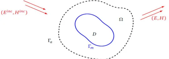
In this paper we focus on the study of the solution of the problem posed either with an absorbent boundary condition or an exact transparent condition:

We denote by and the electric field and the magnetic field of the incident wave, respectively.

Fig. 1 Diffraction of an electromagnetic wave in the presence of an obstacle D where its boundary is noted Γ

The hyperbolicity of Maxwell’s system is immanent, the physical interpretation of this characterization is that the waves and the associated energy propagate in finite time according to particular directions. This property has been little exploited for the resolution of Maxwell’s system whereas it has been widely used for the Euler system, for example. The essential application of this property for numerical computation is the construction of decentred schemes which naturally take into account the direction of propagation of the waves.

In this work, we study to investigate the propagation of a wave emitted in the presence of an obstacle D.

This work is devoted to particular solutions, harmonic in time, this phenomenon is modeled by the the following equations:

∇× + = ℝ ⟍ ,

∇× − = 0 ℝ ⟍ . (3)

For simplicity we assume that J=0.

The idea of solving our problem in the present paper, is to limit the computational domain by a fictitious boundary and using an absorbant condition on this boundary and to use an exact condition on the fictitious boundary, hence the idea of the use of the expression of electric and magnetic fields defined by Stratton-Shu formulas, in the Silver-Müller conditions.

At this phase, we introduce the equations of our problem (4)

⎩ ⎪ ⎨ ⎪

⎧ ,_{− ∇× = 0} ∈ (∇×,Ω) _Ω ℎ :

+∇× = 0 Ω × =− × Γ

× − × ( × ) = ×ℜ( )− × ( ×ℜ( )) Γ

(4)

we set:

= , = , = =

We are going to give a global equation in the vector field W such that: =

Finally the initial problem (4) will be written in this matricial form:

+ . ( ) = 0 =− = ℜ( ) .

(5)

which is equivalent to:

+ + + = 0 Ω ( − )( + ) = 0 Γ

( − )( − ℜ( )) = 0 Γ .

(6)

©IJRASET: All Rights are Reserved

733

0 ×

where for ∈{1,2,3} a vector = , =

0 −

− 0

− 0

Furthermore, = + + .

and denote the positive and negative parts of 1. We also define | | = − . The matrices et , are then

defined by:

= 0 ×

− 0 × and = | |

= − , = −

B. Discretization

The domain Ω is partionned into tetrahedral elements. We denote by the set of elements . We introduce the following space

= { ∈[ ( )] ; | = ∈ ( )}; for all ∈ } where ( ) = {polynomials for of degree ⩽ }.

We denote by = ( , ) the approximate solution of our problem ∈ × and we will define =⋃ ∈ ∩ , =

⋃ ∈ ∩ , =⋃ ∈ ∩ .

Multiplying the equation: +∑_{∈{ , , }} = 0 of the last system by ∈ × and then integrated over an element

∈

( ) + (

∈{ , , }

) = 0

⇔ ( ) + (

∈{ , , }

) = 0

By using Green formula, we have:

( ) − (

∈{ , , }

) + ( ( ) . ) = 0,

Our aim is to find ∈ × which verifies the following equation:

∀ ∈ × , ∫ ( ) − ∫ (∑_{∈{ , , }} ) +∫ ( ( ) . ) = 0, (6)

In the equation (6), we find that there is a term defined on the boundary of the element , but the value is not defined on its faces.

There is the idea of the approach by an approximation of the value of the solution on each edge depending on the right and left traces.

By a development similar to that adopted by Ern and Guermond [12, 13], and adding the terms of the integral representation following formulation is obtained:

∀ ∈ × , an element of obtained:

Find ∈ × such as:

.

∫ ( ) − ∫ (∑_{∈{ , , }} )

+ ∫_∈ ( ) + ( { })

+ ∫_∈ ( ( , + ) )

− ∫_∈ ( ( , − )ℜ( ))

+ ∫_∈ ( ( , + ) )

= ∫_∈ ( ( , − ) )

(9)

where:

represents the incidence matrix between facing surfaces and elements whose entries are given by:

1

©IJRASET: All Rights are Reserved

734

1 ∈ ℎ , −1 ∈ ℎ , 0 ℎ ℎ .

where: is the unitary normal associated to the oriented face and is the unitary normal associated to the cell .

We also define respectively the jump⟦.⟧ and average {. } of a vector to × on the face shared between two elements and

⟦ ⟧= | + | { } = | + |

In this study, we consider two classical numerical fluxes, which lead to different definitions for matrices et , :

1) Centered flux: In this case, = 0 and the faces of the boundary we use

, =

⎩ ⎪ ⎨ ⎪

⎧ 0 ×

− 0 ×

∈ Γ .

| | ∈ Γ .

2) Upwind flux In this case,

=

0 ×

0 ×

; , =

⎩ ⎪ ⎨ ⎪ ⎧

− 0 ×

∈ Γ .

| | ∈ Γ ,

for a homogeneous medium, = = =

Finally, we introduce = ∩ , = ∩ Γ , = ∩ Γ and : the set of indices of neighboring elements of . So we

can write our formulation in the following form:

∀ ∈ × and for an element of :

Find ∈ × such as:

∫ ( ) − ∫ (∑_{∈{ , , }} )

+ ∑_∈ ∫ ( ( + ) )

+ ∑∈ ∫ ( ( + ) )

+ ∫ ( ( , + ) )

− ∫ ( ( , − )ℜ( ))

+ ∫ ( ( , + ) )

= ∫ ( ( , − ) )

where:

= 1 Γ ∩ =

0 Γ ∩ =⌀ =

1 Γ ∩ = 0 Γ ∩ =⌀

©IJRASET: All Rights are Reserved

735

we can reduce our problem as a linear system:

( − ) =

such as is the square matrix of size:

= 6 × ×

this matrix is a sparse matrix defined by block size (6 × 6 ) such as: for = 1, … , : ( , ) = − + × +

× + × and for , = 1, , : ( , ) = ×

with:

=

0 ∩ =⌀

1

also, is a square matrix of the same size as , defined by block size 6 × 6 such as: for , = 1, … , : ( , ) =− ×

× where:

=

0 ∩ =⌀

1

is the vector of size , Where its components are the unknowns of our problem and is the vector of size such as:

( ) = × .

where: = ( ⊗ ), =∑ ⊗ , = ⊗ ( , + ) ,

= ⊗ ( , + ) , = ⊗ ( + ) , =∑∈ ⊗ ( + ) ,

= ⊗ ⊗ , = = ⊗ ( , − ) .

IV.NUMERICALSTUDY

This section is devoted to the numerical resolution of Maxwell’s 3D equations in parallel mode detailed in [17].

Since the linear system resulting from the discretization is of very large size and it is implies complex coefficient blocks and generally, not hermitian, for its resolution, an idea proposed by [38], it is to adopt a decomposition approach Domain. Then the global problem is decomposed into sub-problems related to each other by specific interface conditions.

We consider here an iterative method of Krylov type as a strategy of resolution. Various methods of this type specified in not symmetric matrices (see [37]). In this study, we chose a bi-conjugated stabilized gradient method (BiCGStab) in the numerical tests of this manuscript. The BiCGStab method is introduced in 1992 by van der Vorst [40] and that combines the advantages of BiCG (Bi-Conjugated Gradient) and GMRES methods (see [36]). Following the mathematical study, developed in the previous chapter, of the resolution of the Maxwell equations in unbounded domain by the CDGIR method, we present a sample of the numerical results. We will give some numerical results by making the comparison between the approximate solution and the exact solution. We introduce the error formula:

Error = || − || ( )+ || − || ( )

©IJRASET: All Rights are Reserved

736

Let us consider the problem of the diffraction of a plane wave

Figure 2: Meshing of the volume between a first sphere of

radius = 1 and a second sphere of radius = 1.06. A

mesh size ℎ= 0.07

Figure 3: Meshing of the volume between a first sphere of

radius = 1 and a second sphere of radius = 1.06. A

mesh size ℎ= 0.07.

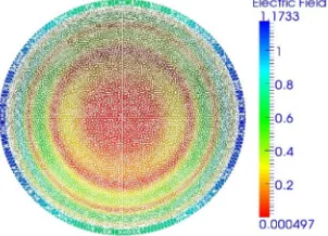
Figure 4: Maxwell 3D equations: diffraction of a plane wave by a perfectly conducting sphere: Approximate solution,

wave number = 5.

Figure 5: Maxwell 3D equations: diffraction of a plane wave by a perfectly conducting sphere: Exact solution, wave

number = 5.

TABLEI

VARIATIONOFEXTERNALRADIUS,K=5

Mesh #M1 #M2 #M3

Distance between and 0.2 0.4 0.6

0.1 0.1 0.1

Number of elements 204222 476454 830879

Relative error (DG) 0.467 × 10 0.288 × 10 0.286 × 10

Relative error (DG+IR) 0.843 × 10 0.883 × 10 0.909 × 10

©IJRASET: All Rights are Reserved

737

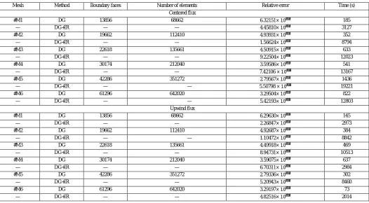
We will study the performances of two methods, Discontinuous Galerkin method and Discontinuous Galerkin method coupled to an integral representation, with the centered and upwind flux according to degree of freedom.

We will fix:

1) The distance between Γ and Γ at 0.5m.

2) A frequency f = 300MHz.

The comparison results between the two methods DG+IR and DG are illustrated in table II in the form of the relative error between the exact solution and the approximate solution either using a centered flux (see also figure 7) or an upwind flux (see also figure 8).

Fig. 7 Electric Field Error according to degree of freedom: Centered flux

Fig. 8 Electric Field Error according to degree of freedom: Upwind flux

TABLEII.PERFORMANCEOFDGANDDG+IRMETHODSWITHCENTEREDANDUPWINDFLUX.

Mesh Method Boundary faces Number of elements Relative error Time (s)

Centered flux

#M1 DG 13856 68662 6.32151× 10 185

— DG+IR — — 4.45810× 10 3127

#M2 DG 19662 112410 4.93931× 10 352

— DG+IR — — 1.56624× 10 8794

#M3 DG 22618 135661 4.50915× 10 633

— DG+IR — — 9.22504× 10 12023

#M4 DG 30174 212040 3.59586× 10 541

— DG+IR — — 7.42106 × 10 13167

#M5 DG 42286 351272 2.79567× 10 1436

— DG+IR — — 5.50798 × 10 19221

#M6 DG 61296 642020 3.29504× 10 822

— DG+IR — — 5.42193× 10 12803

Upwind flux

#M1 DG 13856 68662 6.29630× 10 145

— DG+IR — — 2.26847× 10 2973

#M2 DG 19662 112410 4.92687× 10 384

— DG+IR — — 1.10472× 10 8842

#M3 DG 22618 135661 4.49918× 10 469

— DG+IR — — 8.94731× 10 10513

#M4 DG 30174 212040 3.59075× 10 637

— DG+IR — — 6.70311× 10 2984

#M5 DG 42286 351272 2.79336× 10 302

— DG+IR — — 5.20943× 10 8460

#M6 DG 61296 642020 3.29197× 10 73

— DG+IR — — 4.82516× 10 2014

©IJRASET: All Rights are Reserved

738

We are interested in the case where the discretization step h and the waves number k=10 are fixed and by varying the distance

delimited between the boundary of the obstacle Γ and the artificial boundary Γ by keeping a choice of wavelength equal to 20h.

We will illustrate in a table III the evolution of the error for the two methods DG and DG+IR.

Fig. 9 Error according the size of the domain R

TABLEIII

VARIATIONOFEXTERNALRADIUS,K=5

Mesh Method Distance between and Number of elements Relative error Time (s)

#M1 DG 0.03 0.03 359487 0.380453 × 10 1280

— DG+IR — — — 0.514891 × 10 18271

#M2 DG 0.06 0.03 748447 0.285759 × 10 2370

— DG+IR — — — 0.501781 × 10 34483

#M3 DG 0.12 0.03 897438 0.273918 × 10 2343

— DG+IR — — — 0.500574 × 10 35847

C. Error Depending on the Waves Number

By fixing the number of finite elements layers with two layers, we are interested in the evolution of the error by varying the waves number k and by keeping a choice of wavelength equal to 10h.

We will illustrate in a table IIV the evolution of the error for the two methods DG and DG+IR.

TABLEIIIV

ERROR ACCORDING THE WAVE NUMBER

Mesh Method Wave number Distance between

and

Number of elements

Relative error

Time (s)

#M1 DG 1 1.2 0.6 6901 0.272 × 10 919

— DG+IR — — — — 0.920 × 10 13967

#M2 DG 2 0.57 0.3 18352 0.443 × 10 761

— DG+IR — — — — 0.904 × 10 13221

#M3 DG 8 0.105 0.07 510289 0.353 × 10 3002

— DG+IR — — — — 0.811 × 10 55002

#M4 DG 12 0.08 0.05 1011662 0.251 × 10 5501

— DG+IR — — — — 0.804 × 10 93364

#M5 DG 16 0.054 0.03 800790 0.282 × 10 4009

©IJRASET: All Rights are Reserved

739

Figure 10: Error according the wave number .

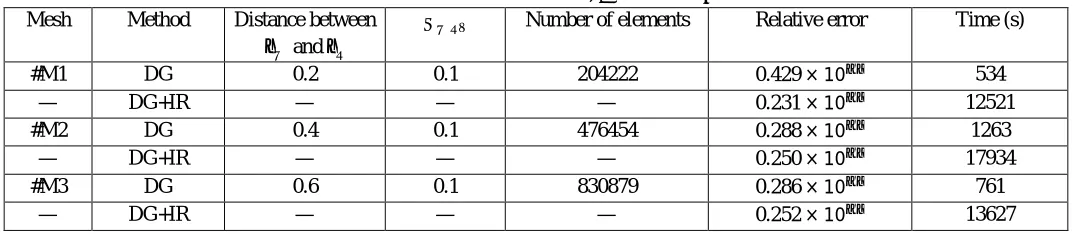
D. Variation of R where =

The table (V) illustrates the results of comparison, of two methods DG and DG+IR, obtained by varying the outer radius and fixing the mesh size h.

TABLEV

VARIATION OF EXTERNAL RADIUS,ℎ= 0.1 AND = 5

Mesh Method Distance between

and

Number of elements Relative error Time (s)

#M1 DG 0.2 0.1 204222 0.429 × 10 534

— DG+IR — — — 0.231 × 10 12521

#M2 DG 0.4 0.1 476454 0.288 × 10 1263

— DG+IR — — — 0.250 × 10 17934

#M3 DG 0.6 0.1 830879 0.286 × 10 761

— DG+IR — — — 0.252 × 10 13627

From the results obtained, it is clear that:

1) The DG+IR method is more efficient.

2) It is clear that the results obtained using the upwind flus are better.

V. CONCLUSION

In study, we have shown the high efficiency of the DG+IR method. So, since the results obtained are encouraging, the contributions proposed in this paper for the 3D Maxwell’s equations aim to make a study with a high interpolation order and to think about the use of other linear system solvers and even to choose a preconditioner in order to to further improve these results

REFERENCES

[1] A. Bendali, Y. Boubendir, and M. Fares. A FETI-like domain decomposition method for coupling finite elements and boundary elements in large-size problems of acoustic scattering. Computers and Structures, 85(9):526 – 535, 2007. High Performance Computing for Computational Mechanics.

[2] Faker Ben Belgacem, Nabil Gmati, and Faten Jelassi. Convergence bounds of GMRES with Schwarz’ preconditioner for the scattering problem. International Journal for Numerical Methods in Engineering, 80(2):191–209, 2009.

[3] Faker Ben Belgacem, Nabil Gmati, and Faten Jelassi. Total overlapping Schwarz’ preconditioners for elliptic problems. ESAIM: M2AN, 45(1):91–113, 2011.

[4] F. Ben Belgacem, M. Fournié, N. Gmati, and F. Jelassi. On the schwarz algorithms for the elliptic exterior boundary value problems. ESAIM: Mathematical Modelling and Numerical Analysis, 39(4):693–714, 2010.

[5] F. Ben Belgacem, N. Gmati, M. Fournié, and F. Jelassi. On Handling the Boundary Conditions at the Infinity for Some Exterior Problems by the Alternating Schwarz Method, pages 325–330. Springer Berlin Heidelberg, Berlin, Heidelberg, 2003.

[6] Pierre Bonnet. Résolution des équations de Maxwell instationnaires et harmoniques par une technique de volumes finis. Application à des problèmes de comptabilité électromagnétique. PhD thesis, 1998. Thèse de doctorat dirigée par FONTAINE, JACQUES Sciences appliquées Clermont Ferrand 2 1998. [7] D. Colton and R. Kress. Inverse Acoustic and Electromagnetic Scattering Theory. Springer Verlag, 1997.

[8] Eric Darrigrand. Couplage Méthodes Multipôles - Discrétisation Microlocale pour les équations Intégrales de l’Electromagnétisme. thèse, Université Sciences et Technologies - Bordeaux I, September 2002.

©IJRASET: All Rights are Reserved

740

[10] Stylianos Dosopoulos and Jin-Fa Lee. Interconnect and lumped elements modeling in interior penalty discontinuous Galerkin time-domain methods. Journal of Computational Physics, 229(22):8521 – 8536, 2010.

[11] M. El Bouajaji and Stéphane Lanteri. High order discontinuous Galerkin method for the solution of 2d time-harmonic Maxwell’s equations. Applied Mathematics and Computation, 219(13):7241–7251, 2013.

[12] A. Ern and J.-L. Guermond. Discontinuous Galerkin methods for Friedrichs systems I. General theory. SIAM J. Numer. Anal., 44(2):753–778, 2006. [13] A. Ern and J.-L. Guermond. Discontinuous Galerkin methods for Friedrichs systems II. Second-order elliptic PDEs. SIAM J. Numer. Anal., 44(6):2363–

2388, 2006.

[14] Hassan Fahs and Stéphane Lanteri. A high-order non-conforming discontinuous Galerkin method for time-domain electromagnetics. Journal of Computational and Applied Mathematics, 234(4):1088 – 1096, 2010.

[15] Hassan Fahs. High-Order Leap-Frog Based Discontinuous Galerkin Method for the Time-Domain Maxwell Equations on Non-Conforming Simplicial Meshes. Numerical mathematics, 2(3):275 – 300, August 2009.

[16] Loula Fezoui, Stéphane Lanteri, Stéphanie Lohrengel, and Serge Piperno. Convergence and stability of a discontinuous Galerkin time-domain method for the 3d heterogeneous Maxwell equations on unstructured meshes. ESAIM: Mathematical Modelling and Numerical Analysis, 39(6):1149–1176, 11 2005. [17] Hugo Fol. Méthodes de type Galerkin discontinu pour la résolution numérique des équations de Maxwell 3D en régime harmonique. PhD thesis, Ecole

Doctorale Sciences Fondamentales et Appliquées, 2006

[18] M. Haddar, F. Chaari, M. Taktak, and T. Boukharrouba. Special issue: Applied acoustics in multiphysic systems preface. Applied Acoustics, 108:1–2, 2016. [19] C. Hazard and M. Lenoir. On the solution of time-harmonic scattering problems for Maxwell’s equations. SIAM Journal on Mathematical Analysis,

27(6):1597–1630, 1996.

[20] Philippe Helluy. Numerical resolution of the harmonic Maxwell equations by a discontinuous Galerkin finite element method. PhD thesis, Ecole nationale superieure de l’aeronautique et de l’espace, 1994.

[21] J.S Hesthaven and T Warburton. Nodal high-order methods on unstructured grids. Journal of Computational Physics, 181(1):186 – 221, 2002.

[22] JS Hesthaven and T Warburton. Discontinuous Galerkin methods for the time-domain Maxwell’s equations. ACES Newsletter, 19(EPFL-ARTICLE-190449):10–29, 2004.

[23] J. S. Hesthaven and T. Warburton. High–order nodal discontinuous Galerkin methods for the Maxwell eigenvalue problem. Philosophical Transactions of the Royal Society of London A: Mathematical, Physical and Engineering Sciences, 362(1816):493–524, 2004.

[24] Ralf Hiptmair. Higher order whitney forms. Progress in Electromagnetics Research, 32:271–299, 2001.

[25] Paul Houston, Ilaria Perugia, and Dominik Schotzau. Mixed discontinuous Galerkin approximation of the Maxwell operator. SIAM Journal on Numerical Analysis, 42(1):434–459, 2005.

[26] A. Jami and M. Lenoir. A variational formulation for exterior problems in linear hydrodynamics. Computer Methods in Applied Mechanics and Engineering, 16(3):341–359, 1978.

[27] J. C. Lin, Shinji Hirai, Chin-Lin Chiang, Wen-Lin Hsu, Jenn-Lung Su, and Yu-Jin Wang. Computer simulation and experimental studies of sar distributions of interstitial arrays of sleeved-slot microwave antennas for hyperthermia treatment of brain tumors. IEEE Transactions on Microwave Theory and Techniques, 48(11):2191–2198, Nov 2000.

[28] Jian Liu and Jian-Ming Jin. A novel hybridization of higher order finite element and boundary integral methods for electromagnetic scattering and radiation problems. IEEE Trans. Antennas and Propagation, 49:1794–1806, 2001.

[29] Peter Monk. Finite Element Methods for Maxwell’s Equations. Oxford University Press, 2003. [30] J.C. Nedelec. Mixed finite elements in ir3 . Numerische Mathematik, 35:315–342, 1980. [31] J.C. Nédélec. Mixed finite elements in R^3. Numerische Mathematik, 35:315–342, 1980.

[32] Ilaria Perugia and Dominik Schotzau. The hp-local discontinuous Galerkin method for low-frequency time-harmonic Maxwell equations. Mathematics of Computation, 72(243):1179–1214, 2003.

[33] Ilaria Perugia, D Schötzau, and P Monk. Stabilized interior penalty methods for the time-harmonic Maxwell equations. Computer Methods in Applied Mechanics and Engineering, 191(41):4675–4697, 2002.

[34] Serge Piperno and Loula Fatima Fezoui. A centered Discontinuous Galerkin Finite Volume scheme for the 3D heterogeneous Maxwell equations on unstructured meshes. Technical Report RR-4733, INRIA, February 2003.

[35] Wm H Reed and TR Hill. Triangular mesh methods for the neutron transport equation. Technical Report LA-UR-73-479, Los Alamos Scientific Laboratory, 1973.

[36] Youcef Saad and Martin H. Schultz. Gmres: A generalized minimal residual algorithm for solving nonsymmetric linear systems. SIAM Journal on Scientific and Statistical Computing, 7(3):856–869, 1986.

[37] Y. Saad. Iterative Methods for Sparse Linear Systems. Society for Industrial and Applied Mathematics, second edition, 2003.

[38] Barry F. Smith, Petter E. Bjorstad, and William D. Gropp. Domain Decomposition: Parallel Multilevel Methods for Elliptic Partial Differential Equations. Cambridge University Press, New York, NY, USA, 1996.

[39] Guillaume Sylvand. La méthode multipôle rapide en électromagnétisme. Performances, parallélisation, applications. thèses, Ecole des Ponts ParisTech, June 2002.

[40] H. A. van der Vorst. Bi-cgstab: A fast and smoothly converging variant of bi-cg for the solution of nonsymmetric linear systems. SIAM Journal on Scientific and Statistical Computing, 13(2):631–644, 1992.

[41] Dong Xue, Leszek Demkowicz, et al. Control of geometry induced error in hp finite element (fe) simulations. i. evaluation of fe error for curvilinear geometries. Int. J. Numer. Anal. Model, 2(3):283–300, 2005.