Performane Improvement of Indoor and Outdoor
Channel Models in Wireless Networks
Yuvraj Singh Ranawat1, Suraj Kumhar2 1,2
Assistant Professor, Mewar University, Chittorgarh, India
Abstract: A radio propagation model, also known as the radio frequency propagation model, is an empirical mathematical formulation for the characterization of radio wave propagation as a function of frequency, distance and other conditions .A single model is usually developed to predict the behavior of propagation for all similar links under similar constraints. Created with the goal of formalizing the way radio waves are propagated from one place to another, such models typically predict the path loss along a link or the effective coverage area of a transmitter.The channel model can vary with the antenna configuration in the transmitter and receiver (e.g., depending on single antenna system or multiple antenna system). Especially in the recent development of the multi-input and multi-output (MIMO) systems, acompletely different channel model is required to capture their spatio-temporal characteristics(e.g., the correlation between the different paths among the multiple transmit and receive antennas) [24]. This paper surveys different channel models used to characterise wireless indoor and outdoor environment. To develop and validate positioning algorithms under realistic conditions, an accurate knowledge of the propagation channel is significant. An outdoor-to-indoor channel model is proposed based on an extension of the geometry-based stochastic modeling approach to fulfill the requirements. The parameters of the outdoor-to-indoor channel model are extracted from two channel measurement campaigns. The proposed outdoor-to-indoor channel model is capable of accurately simulating the time variant channel. A comparison of the channel model with the channel measurement data is performed by comparing statistics.
Keywords: SISO Channel models, MIMO, Doppler spectrum, Power delay profile (PDP), Doppler power spectrum (PSD).
I. INTRODUCTION
As high-speed data services for multimedia Internet access are brought to focus, huge date rates per user are anticipated for future 3G and 4G mobile radio systems. The most likely method of increasing capacity for wireless transmission is to exploit smart antennas. The algebraic framework is suitable for the description of SISO (single-input-single-output) radio transmission systems [8]. Channel models describe a communication channel and are essential in developing efficient wireless communication networks. The channel model can vary with the antenna configuration in the transmitter and receiver (e.g., depending on single antenna system or multiple antenna system).
Especially in the recent development of the multi-input and multi-output (MIMO) systems, a completely different channel model is required to capture their spatio-temporal characteristics (e.g., the correlation between the different paths among the multiple transmit and receive antennas). Fading properties of indoor wireless channels are quite different from those of mobile (vehicular) channels due to differences in the physical environment and the consequent differences in propagation mechanisms. In mobile wireless channels, 5–10 (and perhaps fewer) most significant paths are usually responsible for more than 80% of power delivered between the transmitter and receiver antennas. Rays along those paths undergo diffraction around vertical or horizontal edges of buildings, reflection off building surfaces, ground reflection, vegetation scattering, and so forth. If the dominant path to the receiver is shadowed by an obstacle, the total power may attenuate significantly, a phenomenon that earlier we called shadow fading.
II. INDOOR CHANNEL MODELS
A. General Indoor Channel Models
In this subsection, we consider the two most popular indoor channel models: 2-ray model and exponential model. In the 2-ray model, there are two rays, one for a direct path with zero delay (i.e., 00), and the other for a path which is a reflection with delay
of 10, each with the same power (see Figure 2.1 for its PDP) [5]. In this model, the maximum excess delay is m1 and the
mean excess delay is given as 1
2
. It is obvious that the RMS delay is the same as the mean excess delay in this case (i.e.,
1
2
. In other words, the delay of the second path is the only parameter that determines the characteristics of this particular
model. However, it might not be accurate, simply because a magnitude of the second path is usually much less than that of the first path in practice. This model may be acceptable only when there is a significant loss in the first path.
In the exponential model, the average channel power decreases exponentially with the channel delay as follows:
(2.1)
where d is the only parameter that determines the power delay profile (PDP). Figure 2.1 illustrates a typical PDP of the exponential
model. This model is known to be more appropriate for an indoor channel environment. The mean excess delay and RMS delay spread turn out to be equal to each other, that is, dand d, in the exponential model. Meanwhile, the maximum excess
delay is given as
m dlnA (2.2)
Figure 2.1 2-ray model vs. exponential model: an illustration.
where A is a ratio of non-negligible path power to the first path power, that is, AP
m / P(0)exp(m/d). Note that Equation(2.1) can be represented by the following discrete-time model with a sampling period of Ts
max
1
(p) pTs , p 0,1,..., p
P e
(2.3)
where p is the discrete time index with pmax as the index of the last path, that is, pmax[m/Ts] . A total power for the PDP in
Equation (2.3) is given as
max 1 max 0 1 1 (p) . 1 s s T p p total T p e P P e
(2.4)In order to normalize the total power in Equation (2.4) by one, Equation (2.3) has been modified as
(0) e , 0,1,... max spT
P p P p p (2.5)
where P(0) is the first path power.
1 dB. IEEE 802.11 Channel Model
IEEE 802.11b Task Group has adopted the exponential model to represent a 2.4 GHz indoor channel [23]. Its PDP follows the exponential model as shown in Section 2. A channel impulse response can be represented by the output of finite impulse response (FIR) filter. Here, each channel tap is modeled by an independent complex Gaussian random variable with its average power that follows the exponential PDP [4], while taking the time index of each channel tap by the integer multiples of sampling periods. In other words, the maximum number of paths is determined by the RMS delay spread st and sampling period Ts as follows:
pmax[10. / T ]s (2.6)
Assuming that the power of the pth channel tap has the mean of 0 and variance of 2
/ 2 p
, its impulse response is given as
hpZ1 j Z p. 2, 0,...,pmax (2.7)
where Z1 and Z2 are statistically independent and identical Gaussian random variables, each with 2
(0, p/ 2)
N .
As opposed to the exponential model in which the maximum excess delay is computed by a path of the least non-negligible power level, the maximum excess delay in IEEE802.11 channel model
is fixed to 10 times the RMS delay spread. In this case, the power of each channel tap is given as 2 2 /
0 s
pT
p e
(2.8)
where 2 0
is the power of the first tap, which is determined so as to make the average received
power equal to one, yielding
max
/ 2
0 1 /
1 1
s s
T
p T
e e
(2.9)
In the IEEE 802.11 channel model, a sampling period Ts must be at least as small as 1/4. Figure 2.2 shows the average channel power and channel frequency response for the IEEE 802.11 channel model. Since the RMS delay spread is relatively small in this example, the power variation in the frequency domain is within at most 15dB, which implies that frequency selectivity is not that significant [22].
(a) Average channel power (b) Channel frequency response Figure 2.2 IEEE 802.11 channel model.
C. Saleh-Valenzuela (S-V) Channel Model
It has been verified by intense measurements of the indoor channel that arrivals of the multipathdelayed components can bemodeled as a Poisson process. More specifically, Saleh and Valenzuela have proposed a new channel model (referred to as S-V channel model) after finding from the indoor channel measurements that there are multiple clusters, eachwithmultiple rays, in the delay profile [24].
The S-V channel model with multiple clusters, each of which is associated with a set of rays. The arrival times of each cluster as well as rays in each cluster follow an individual Poisson process. Therefore, the delay of each path is not spaced in the multiple of sampling periods, but spaced in a rather arbitrary manner [24]. More specifically, the arrival time of the first ray in the mth cluster, denoted by Tm, is modeled by a Poisson process with an average arrival rate of while the arrival times of rays in each cluster is
fTm
T Tm m1
exp[
TmTm1
], m1, 2,.... (2.10)and
fr m,
r m, r1 ,m
exp[
r m, r1 ,m
], r1, 2,.... (2.11)where r m, denotes the arrival time of the rth ray in the mth cluster. In Equation (2.10) and Equation (2.11), the arrival time of the
first ray in the mth cluster, 0,m, is defined as the arrival time of themth cluster, Tm (i.e.,0,mTm). Let r,mand r,mdenote amplitude
and phase of the rth ray in the mth cluster, respectively. Then, a channel impulse response is given as
,
, ,
0 0 r m
j
r m m r m
m r
h t e t T
(2.12)where r,m is a random variable that is uniformly distributed over
0, 2
and r,mis an independent random variable with thefollowing Rayleigh distribution:
2 2, ,
,
/ 2
, , 2 , /
r m r m
r m r m r m r m
f e
(2.13)
In Equation (2.13), r m, is the average power of the rth ray in the mth cluster, which is given as
2 2 / , /
, 0,0
r m m
T
r m e e
(2.14)
where and denote time constants for exponential power attenuation in the cluster and ray, respectively, while 2 0,0
denotes the
average power of the first ray in the first cluster [21]. the S-V channelmodel is a double exponential delay model in which average cluster power decays exponentially by following a term eTm/ in Equation (2.14 )while average ray power in each cluster also
decays exponentially by following a term r m, /
e in Equation (2.14). Once the average power of the first ray in the first cluster, 2 0,0 ,
is given, the average power of the rest of rays can be determined by Equation (2.14), which subsequently allows for determining the Rayleigh channel coefficients by Equation (2.13). In case that a path loss is not taken into account, without loss of generality, the average power of the first ray in the first cluster is set to one. Even if there are an infinite number of clusters and rays in the channel impulse response of Equation (2.12), there exist only a finite number of the non-negligible numbers of clusters and rays in practice. Therefore, we limit the number of clusters and rays to M and R, respectively. Meanwhile, a log-normal random variable X, that is,
2
10
20log X N 0, x , can be introduced to Equation (2.12), so as to reflect the effect of long-term fading as
,
, ,
0 0 r m
M R
j
r m m r m
m r
h t X e t T
[image:4.612.86.526.458.718.2]
(2.15)Figures 2.3 show the distributions of cluster arrival times and ray arrival times, respectively, including the simulation results to be comparedwith the analytical ones where the mth cluster arrival time Tm and the rth ray arrival time r m, in the mth cluster are
generated in such a way that each of them has an exponential distribution of Equation (2.10) and Equation (2.11), respectively. Figure 2.3 shows the channel impulse response of theS-V channel. Figure 2.3, showing the channel power distribution, is obtained by simulating 1,000 channels, from which it is clear that the channel power follows a log-normal distribution [20].
D. UWB Channel Model
According to measurements of broadband indoor channel, it has been found that amplitudes of multipath fading follow the log-normal or Nakagami distribution rather than the Rayleigh distribution, even if they also show the same phenomenon of clustering as in the Saleh- Valenzuela (S-V) channel model. Based on these results, SG3a UWB multipath model has been proposed by modifying the S-V model in such a way that the cluster signals are subject to independent log-normal fading while the multi-path signals in each cluster are also subject to independent log-normal fading [25].
The ith sample function of a discrete-time impulse response in the UWB multi-path channel model is given as
,
,
0 0M R
i i i
i i r m m r m
m r
h t X a t T
(2.16)where , , , ,
i i
i r m r m
X a T and ,
i r m
are defined as the same as in Equation (2.15), nowwith the index i to represent the ith generated
sample function of the channel. For simplicity of exposition, the index i in Equation (2.16) will be eliminated in the following discussion. As in the S-V channel model, the arrival time distributions of clusters and rays are given by two different Poisson processes of Equation (2.10) and Equation (2.11), respectively. The UWB channel model is different from the S-V channel model in that clusters and rays are subject to independent log-normal fading rather than Rayleigh fading. More specifically, a channel coefficient is given as
r m, pr m m, r m, (2.17)
where m represents log-normal fading of the mth cluster with the variance of
2 1
while r m, represents log-normal fading of the
rth ray with the variance of 2 2
in the mth cluster. Note that independent fading is assumed for clusters and rays. In Equation (2.17),
,
r m
p is a binary discrete random variable to represent an arbitrary inversion of the pulse subject to reflection, that is, taking a value
of +1 or -1 equally likely. As compared to the channel coefficients of the S-V channel model in Equation (2.12) which has a uniformlydistributed phase over
0, 2
, those of UWB channel model have the phase of either or , making the channel coefficient always real [14]. Furthermore, we note that amplitude of each ray is given by a product of the independent log-normal random variables, m and r m, . Since a product of the independent log-normal random variables is also a log-normal randomvariable, a distribution of the channel coefficient , 1 2/ 20
, 10 r m z z
m r m
also follows a log-normal distribution, that is,
2 2
10 , , 1 2
20log ( m r m) N r m, , with its average power given as
2 / , /
, 0
r m m
T
m r m
E e e
(2.18)
where 0 represents the average power of the first ray in the first cluster.Meanwhile, mean of the channel amplitude for the rth ray
in the mth cluster can be found as
2 2
1 2
0 ,
,
ln 10
10ln 10 / 10 /
ln 10 20
m r m
r m
T
(2.19)
Besides the same set of channel parameters as in the S-V channel model, including the cluster arrival rate , ray arrival rate , cluster attenuation constant , ray attenuation constant , standard deviation x of the overall multipath shadowing with a
channel h(t) in Equation (2.16) is given as a real number. Some proper modifications such as downconversion and filtering are required for implementing the UWB channel in simulation studies, since its bandwidth cannot be limited due to arbitrary arrival times. All the channel characteristics for UWB channel model, including mean excess delay, RMS delay spread, the number of significant paths within 10dB of peak power (denoted as NP10dB), and PDP, must be determined so as to be consistent with the
measurements in practice.
Target channel characteristics CM1 CM2 CM3 CM4
Mean excess delay (nsec)
5.05 10.38 14.18RMS delay (nsec)
5.28 8.03 14.28 2510dB
NP 35
NP(85%) 24 36.1 61.54
Model parameters
(1/nsec) 0.0233 0.4 0.0667 0.0667
(1/nsec) 2.5 0.5 2.1 2.1
7.1 5.5 14.00 24.00
4.3 6.7 7.9 12
1
(dB) 3.3941 3.3941 3.3941 3.3941
2
(dB) 3.3941 3.3941 3.3941 3.3941
x
(dB) 3 3 3 3
Model parameters
Mean excess delay (nsec)
5.0 9.9 15.9 30.1RMS delay (nsec)
5 8 15 2510dB
NP 12.5 15.3 24.9 41.2
NP(85%) 20.8 33.9 64.7 123.3
Channel energy mean (dB) -0.4 -0.5 0.0 0.3
[image:6.612.64.542.142.562.2]Channel energy std (dB) 2.9 3.1 3.1 2.7
Table 2.1 UWB channel parameters and model characteristics [25].
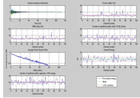
Figure 2.4 Generation of UWB channel: example (CM1).
Figure 2.4 shows UWB channel model are used to set the UWB channel parameters as listed in Table 2.1, to convert the continuous-time UWB channel into the corresponding discrete-continuous-time one, and to generate a UWB channel model, respectively. It shows the UWB channel characteristics by simulating 100 CM1 channels. Here, the sampling period has been set to 167 ps. In the current measurement, the RMS delay spread turns out to be around 5 ns, which nearly coincides with the target value of CM1 channel in Table 2.1. The same observation is made for the mean excess delay [24].
III. OUTDOOR CHANNEL MODELS
As opposed to the static or quasi-static nature of the indoor channel, outdoor channels are typically characterized by time variation of the channel gain, which is subject to the mobile speed of terminals. Depending on the mobile speed, time variation of channel gain is governed by Doppler spectrum, which determines the time-domain correlation in the channel gain. In this subsection, we discuss how to model the time-correlated channel variation as the mobile terminal moves. Furthermore, we present some practical methods of implementing the outdoor channel models for both frequency-flat and frequency-selective channels.
A. FWGN Model
The outdoor channel will be mostly characterized by Doppler spectrum that governs the time variation in the channel gain. Various types of Doppler spectrum can be realized by a filtered white Gaussian noise (FWGN) model. The FWGN model is one of the most popular outdoor channel models. The Clarke/Gans model is a baseline FWGN model that can be modified into various other types, depending on how a Doppler filter is implemented in the time domain or frequency domain.We first discuss the Clarke/Gans model and then, its frequency-domain and time-domain variants.
component is subject to Doppler shift. Finally, the Doppler-shifted Gaussian noise is transformed into the time-domain signal via an IFFT block. Since output of the IFFT block must be a real signal, its input must be always conjugate symmetric. Constructing a complex channel gain by adding a real part to an imaginary part of the output, a channel with the Rayleigh distributed-magnitude is generated.
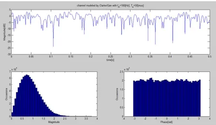
Figure 3.2 shows the time-domain characteristics of the frequency-non-selective fading channel with a Doppler frequency of 100
m
f Hzand a sampling period of Ts50s. From these results, it is observed that the channel gain is time-varying with the Rayleigh-distributed amplitude and uniformly-distributed phase. Variation of the channel amplitude becomes more significant as the Doppler frequency increases, demonstrating the fast fading characteristics
(t) I
h
h(t)hI(t)jhQ(t)
(t) Q
[image:8.612.47.538.198.399.2]jh
Figure 3.1 Block diagram for Clarke/Gans model.
Figure 3.2 Generation of a time-varying channel with Clarke/Gans model. (a) Time-domain channel characteristics (b) Distribution of magnitude (c) Distribution of phase
Complex Gaussia
n noise
IFFT
IFFT Complex
Gaussian noise
[image:8.612.82.529.428.687.2]2) Modified Frequency-Domain FWGN Model: Since the Clarke/Gans model employs two IFFT blocks, it has disadvantages of computational complexity. Among many other variants of the Clarke/Gans model, we here describe one used in I-METRA model.
Figure 3.3 describes a process of generating the Doppler spectrum. Let fmdenote the Doppler frequency. Since the spectrum repeats
with respect to Nyquist frequency, 2fm, for normal sampling, it must be folded for an IFFT function to deal with the positive
frequency components only as shown in Figure 3.3(a). When oversampled by a factor of NOS, the bandwidth of Doppler spectrum
becomesBD2N fos mas shown in Figure 3.3(b). Its inverse 1 D
t B
is the sample spacing in the time domain, which corresponds to
the coherence time of the fading channel. Dividing the Doppler bandwidth into NFading subbands, each subband of the length
/
m D Fading
f B N
leads to the overall length of the fading channel, given by 1 /
Fading Fading D
m
T N B
f
. Meanwhile, Figure 3.3(c)
shows a discrete-frequency Doppler spectrum and its equivalent discretetime fading channel. For the IFFT size of NFading, the
frequency spacing of Doppler spectrum is
Folding
m
f
fm 0 fm 2fm
(a) Normal sampling
2 os m
B N f TFading1 f 1
B NFading
Fourier transform
f t
fm N fos m 2N fos m 0
t 1B01 2
N fos m
(b) Oversampling
/ 2
m D Fading os Fading
f B N N f N
D m Fading
B f N TFading1 f 1
B NFading
IFFT/FFT
ND1 NFading1
ND fm fmNFading
2Nos
t 1B01 2
N fos m
(c) Discrete-time oversampling
Figure 3.3 Generation of Doppler spectrum.
given by fm2N fos m/NFading. The number of discrete-time frequency samples in the overall Doppler spectrum is given by
/ (2 N )
D m m Fading os
N f f N . This particular method allows for generating the fading signal with a given duration of TFading without
taking the maximum Doppler frequency into account. Furthermore, it is advantageous for simulation since the time-domain signal can be obtained by interpolation with the maximum Doppler frequency fm.
0
Here, a magnitude of channel response can be computed from the Doppler spectrum with an arbitrary phase. A channel response of each path in the time domain is given as
2 1
2 2
Fading
Fading k
Fading
N
j nk N
j
k N
h n S k ee
(3.1)where S k
is the Doppler spectrum at a discrete frequency k f fm,ntt is the discrete time index, and k is a uniformrandom variable over
0, 2
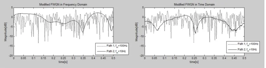
.According to the reports on channel measurements, the different channel environments are subject to the different Doppler spectrumand furthermore, the maximum Doppler frequency as well as Doppler spectrum may vary for each path. Figures 3.4(a) and (b) show two different paths, with the maximum Doppler frequency of 100 Hz and 10 Hz, respectively, which are generated by the modified frequency-domain and time-domain FWGN models with the Classical Doppler spectrum, respectively.
(a) Modified frequency-domain FWGN model (b) Modified time-domain FWGN model Figure 3.4 Generation of two different paths with FWGN channel model.
3) Time-Domain FWGN Model: As shown in Figure 3.5, we can generate the fading channel by filtering the complex Gaussian random process with the time-domain filter whose frequency response corresponds to the Doppler spectrum. Due to the various advantages of the time-domain FWGN model, it is frequently employed in the commercial channel simulators.
[image:10.612.84.534.227.343.2]Fading channel
Figure 3.5 Time-domain FWGN model: an overview.
As opposed to the frequency-domain FWGN model in which the duration of fading channel is determined by the IFFT size of
Fading
N and the frequency-domain oversampling factor of Nos, it is determined by the length of the complex Gaussian random
signal in the time-domain FWGN model. Since the simulation interval can be extended simply by increasing the number of complex Gaussian random samples subject to the Doppler filter, it is flexible for simulation [16].
The FWGN channel model allows for employing various other types of Doppler spectrum, including the flat Doppler spectrum and Laplacian Doppler spectrum. The flat Doppler spectrumhas the constant power spectral density function, i.e.,
S f
1, f fm (3.2)Meanwhile, the Laplacian Doppler spectrum is defined by the following power spectrum density function:
1 1
2
1 2 2
exp cos xp cos ,
1
m m m
m
S f f f e f f f f
f f
(3.3)
where s is the standard deviation of PAS, and f is the difference between direction of movement (DoM) and direction of arrival (DoA). Unlike the flat or classical Doppler spectrum model, the mobile direction can be accounted into the Laplacian Doppler spectrum.
Complex Gaussian generator
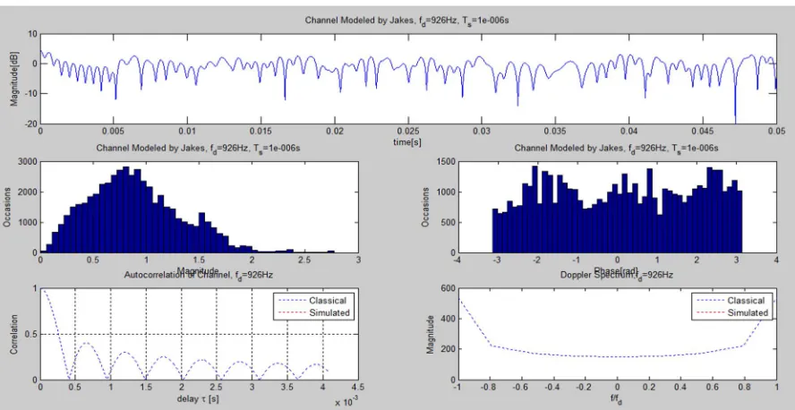
B. Jakes Model
ARayleigh fading channel subject to agivenDoppler spectrumcan begenerated bysynthesizing the complex sinusoids. The number of sinusoids to add must be large enough to approximate the Rayleigh amplitude [24]. Figure 3.6 illustrates how the Jakes model is implemented. It has been assumed that all rays of the scattered components arriving in the uniform directions are approximated by N plane waves. Define N0
N 2 1 2
where N 2 is limited to an odd number. Let un denote an angle of arrival for the nth planewave, which is modeled n2n N, n1, 2,..., N0. As shown in Figure 3.6, a sum of N0 complex oscillator outputs with the
frequencies of wnwdcosn,n1, 2,...,N0, each corresponding to different Doppler shifts, is added to the output of a complex
oscillator with a frequency of wd2fm.
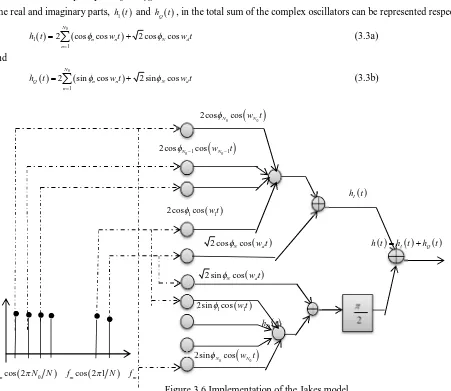
The real and imaginary parts, h t1
and hQ
t , in the total sum of the complex oscillators can be represented respectively as1
0
1
2 cos cos 2 cos cos N
n n N d
n
h t w t w t
(3.3a)and
0
1
2 sin cos 2 sin cos N
Q n n N d
n
h t w t w t
(3.3b)2cosN0cos
w tN0
2cosN01cos
wN01t
I
h t
2 cos1cos
w t1
2 cosNcos
w td
h t
h tI
hQ
t2 sinNcos
w td
2sin1cos
w t1
hQ
t2sinN0cos
w tN0
0
cos 2 m
[image:11.612.48.499.190.581.2]f N N fmcos 2 1
N
fmFigure 3.6 Implementation of the Jakes model.
where n and N are the initial phases of the n-th Doppler-shifted sinusoid and the maximum Doppler frequency fm, respectively.
The number of the Doppler-shifted sinusoids, N0, must be large enough to approximate the amplitude of the fading channel with a Rayleigh distribution. It has been known that N08 is large enough. Note that the following properties can be shown for Equation
(3.3):
2 2
2 0
0 1 0
0 0 2
2 1 2 1
Q
E h t
E h t E
E E
N N
(3.4)
2
2 0E h t
E0 (3.6)E h t h
1
Q t
0 (3.7)Equation (3.5) and Equation (3.6) confirm that the Jake model generates the fading signal with the average amplitude of E0 and
average energy of 2 0
E . Furthermore, Equation (3.4) and Equation (3.7) show that the real and imaginary parts of the channel are
statistically independent with the average power of 2 0 2
[image:12.612.84.528.162.391.2]E .
Figure 3.7 Generation of a time-varying channel with Jakes model. (a) Time-domain channel characteristics (b) Distribution of magnitude (c) Distribution of phase (d) Autocorrelation function (e) Doppler spectrum
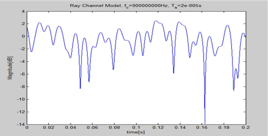
C. Ray-Based Channel Model
A ray-based model is frequently used in modeling a MIMO channel, since it can take a spatiotemporal correlation into account [26]. However, it can be also used for a SISO channel. Its fundamental principle is described in this subsection while its extension to the MIMO channel . As in the Jake’s model, the ray-based model is given by a sum of the arriving plane waves. As shown in Figure 3.8, it can model the plane waves incoming from an arbitrary direction around the mobile terminal, which can deal with the various scattering environments. In general, its power azimuth spectrum (PAS) is not uniform. Unlike the Jakes model, therefore, its Doppler spectrum is not given in the U-shape, but in various forms, depending on the scattering environments.
[image:12.612.85.531.531.720.2]Cluster n
Subpath m
, ,
n m AoA
N
n m AoD, , MS V V
N n m AoA, , n AoA,
MS
n AoA,
MS
, ,
n m AoD
BS
MS array broadside MS array
[image:13.612.90.494.86.255.2]BS array broadside MS direction of travel
Figure 3.9 Ray-based MIMO channel model
Figure 3.9 shows one of the Ray-based channel models, known as a spatial channel model (SCM) for a MIMO channel in 3GPP [28]. Let hu s n, ,
t denote a channel impulse response of the nth path (cluster) between the sth transmit antenna and uth receiveantenna, which can be represented as [28]
, , , ,AoD ,
, ,
1
, , , ,AoA , ,AoA
exp sin
exp sin exp(jk cos t)
M BS n m AoD s n m n m
n SF
u s n
m
MS n m AoA u n m n m v
G j kd
P
h t
M G jkd V
(3.8)where
n
P: power of the nth path
SF
: standard deviation of log-normal shadowing
M: the number of subrays per path
, , AoD
n m
: angle of departure of the mth subray for the nth path
, , AoA
n m
: angle of arrival (AoA) of the mth subray for the nth path
,
n m
: random phase of the mth subray for the nth path
, ,
BS n m AoD
G : BS antenna gain of each array element
, ,
MS n m AoA
G : MS antenna gain of each array element
k: wave number 2 where is the carrier wavelength
s
d : distance between antenna element s and reference antenna element (s=1) in BS
u
d : distance between antenna element u and reference antenna element (u=1)in MS
V : magnitude of MS velocity vector
v
Figure 3.10 Ray-Based Channel with Uniform Power Subray Method
A uniform power subray-based channel model can be generated to get an angle spacing for equal power Laplacian PAS in SCM(spatial channel model), to assign the AoA/AoD offset tomean AoA/AoD, to generate DoAs at BS/MS and a randomphase at BS, and to combine the phases of M subrays to generate complex channel coefficients for each path, respectively
D. SUI Channel Model
According to the IEEE 802.16d channel model , a suburban path loss environment has been classified into three different terrain types, depending on the tree density and path-loss condition. The SUI (Stanford University Interim) channel model deals with the same environment as in the IEEE 802.16d channel model. Using the different combinations of the channel parameters, it identifies six different channel models that can describe the typical three terrain types in North America [9, 10] .The details of the channel parameters for the different SUI models are summarized. Note that the different K-factors and st are set for the different antenna types, for example, directional or omni antennas [9, 10].
Terrain type SUI channels
A SUI-5, SUI-6
B SUI-3, SUI-4
C SUI-1, SUI-2
Table 3.1 SUI channel models for the different terrain types.
In the SUI channel models, the Doppler power spectrum (PSD) is modeled as the following truncated form:
2 4
0 0 0
0
1 1.72 0.785 , 1
0, 1
f f f
S f
f
(3.9)
[image:14.612.73.538.488.553.2]Figure 3.11 Channel characteristics for SUI-6 channel model. (a) Power delay profile (PDP) (b) Time-domain channel characteristic (c) PSD: h1 (d) PSD: h2 (e) PSD: h3
IV. CONCLUSION
In conclusion, it has been verified that the current channel model properly realizes the target channel characteristics. The contribution of this paper is an outdoor-to-indoor channel model fulfilling the requirements for simulations of mobile radio based positioning algorithms. The non-line-of-sight bias and the continuous evolution of multipath components with time are taken into account. A comparison of the channel model with the channel measurement data is performed by comparing statistics.
REFERENCES
[1] Sklar, B. (2002) Digital Communications: Fundamentals and Applications 2/E, Prentice Hall.
[2] Rappaport, T.S. (2001) Wireless Communications: Principles and Practice 2/E, Prentice Hall.
[3] Greenwood, D. and Hanzo, L. (1994) Characterization of mobile radio channels. Chapter 2, Mobile Radio Communications (ed. R. Steele), Pentech Press-IEEE
Press, London.
[4] Friis, H.T. (1946) A note on a simple transmission formula. Proc. IRE, 34(5), 254–256.
[5] Lee, W.C.Y. (1985) Mobile Communications Engineering, McGraw Hill, New York.
[6] Okumura, Y., Ohmori, E., Kawano, T., and Fukuda, K. (1968) Field strength and its variability in VHF and UHF land mobile radio service. Rev. Elec. Commun. Lab., 16, 825–873.
[7] Hata, M. (1980) Empirical formula for propagation loss in land mobile radio services IEEE Trans. Veh. Technol., 29(3), 317–325
[8] Erceg, V., Greenstein, L.J., Tjandra, S.Y. et al. (1999) An empirically based path loss model for wireless channels in suburban environments. IEEE J. Select.
Areas Commun., 17(7), 1205–1211.
[9] IEEE (2007) 802.16j-06/013r3. Multi-Hop Relay System Evaluation Methodology (Channel Model and Performance Metric).
[10] IEEE (2001) 802.16.3c-01/29r4. Channel Models for Fixed Wireless Applications.
[11] IST (2004) 4-027756. WINNER II, D1.1.1 WINNER II Interim Channel Models.
[12] Recommendation (1997) ITU-R M.1225. Guidelines for Evaluation of Radio Transmission Technologies for IMT-2000.
[13] Clarke, R.H. (1968) A statistical theory of mobile radio reception. Bell System Tech. J., 47, 987–1000.
[14] Capoglu, I.R., Li,Y., and Swami, A. (2005) Effect of doppler spread in OFDM based UWB systems. IEEE Trans. Wireless Commun., 4(5), 2559–2567.
[15] Stuber, G.L. (1996) Principles of Mobile Communication, Kluwer Academic Publishers.
[16] Tepedelenliglu, C. and Giannakis, G.B. (2001) On velocity estimation and correlation properties of narrow-band mobile communication channels. IEEE Trans.
Veh. Technol., 50(4), 1039–1052.
[17] Andersen, J.B., Rappaport, T.S., and Yoshida, S. (1995) Propagation measurements and models for wireless communications channels. IEEE Commun. Mag.,
33(1), 42–49.
[18] Bajwa, A.S. and Parsons, J.D. (1982) Small-area characterisation of UHF urban and suburban mobile radio propagation. Inst. Elec. Eng. Proc., 129(2), 102–
109.
[19] Bello, P.A. (1963) Characterization of randomly time-variant linear channels. IEEE Trans. Commun., 11(4), 360–393.
[20] Black, D.M. and Reudink, D.O. (1972) Some characteristics of mobile radio propagation at 836 MHz in the Philadelphia area. IEEE Trans. Veh. Technol., 21(2), 45–51.
[21] Corazza, G.E. and Vatalaro, F. (1994) A statistical model for land mobile satellite channels and its application to nongeo stationary orbit systems systems. IEEE
Trans. Veh. Technol., 43(3), 738–742.
[23] IEEE (1996) P802.11-97/96. Tentative Criteria for Comparison of Modulation Methods.
[24] Saleh, A.M. and Valenzuela, R.A. (1987) A statistical model for indoor multipath propagation. IEEE J. Select. Areas Commun., 5(2), 128–137.
[25] IEEE (2003) 802.15-02/490R-L. Channel Modeling sub-committee. Report finals.
[26] Smith, J.I. (1975)Acomputer generated multipath fading simulation for mobile radio. IEEE Trans. Veh. Technol., 24(3), 39–40.
[27] Jakes, W.C. (1974) Microwave Mobile Communications, John Wiley & Sons, Inc., New York.
[28] 3GPP (2007) TR 25.996, v7.0.0. 3rd Generation Partnership Project; Technical Specification Group Radio Access Network; Spatial Channel Model For
Multiple Input Multiple Mutput Simulations (Release 7).
[29] SCM (2002) 065v2. SCM Model Correlations.
[30] SCM (2002) 033-R1. Spatial Channel Model Issues.
[31] COST 207 (1989) Digital land mobile radio communications, _ECSC-EEC-EAEC, Brussels-Luxembourg,1989.
[32] Fleury, B.H. and Leuthold, P.E. (1996) Radiowave propagation in mobile communications: An overview of European research. IEEE Commun. Mag., 34(2),
70–81.
[33] Greenstein, L.J. (1978) A multipath fading channel model for terrestrial digital radio systems. IEEE Trans. Commun., 26(8), 1247–1250.
[34] Loo, C. (1985) A statistical model for a land mobile satellite link. IEEE Trans. Veh. Technol., 34(3), 122–127.
[35] Lutz, E. and Plochinger, E. (1985) Generating Rice processes with given spectral properties. IEEE Trans. Veh. Technol., 34(4), 178–181.
[36] Schilling, D.L. et al. (1991) Broadband CDMA for personal communications systems. IEEE Commun. Mag., 29(11), 86–93.
[37] Seidel, S.Y. et al. (1991) Path loss, scattering and multipath delay statistics in four european cities for digital celluarl and microcellular radiotelephone. IEEE
Trans. Veh. Technol., 40(4), 721–730.
[38] Pedersen, K.I., Mogensen, P.E., and Fleury, B.H. (2000) A stochastic model of the temporal and azimuthal dispersion seen at the base station in outdoor propagationenvironments. IEEE Trans. Veh. Technol., 49(2), 437–447.
[39] Schumacher, L., Pedersen, K.I., and Mogensen, P.E. (2002) From antenna spacings to theoretical capacitiesguidelines for simulating MIMO systems.
PIMRC’02, vol. 2, pp. 587–592.

![Table 2.1 UWB channel parameters and model characteristics [25].](https://thumb-us.123doks.com/thumbv2/123dok_us/1242406.650335/6.612.64.542.142.562/table-uwb-channel-parameters-model-characteristics.webp)