Performance Analysis of Supervised Remote Sensing Methods for Forest Identification in Pakistan

Performance Analysis of Supervised Remote

Sensing Methods for Forest Identification in

Pakistan

Ahmad Junaid1, Nasru Minallah2, Afnan H. Khan3, Muftooh UR Rehman4, Riaz Muhammad5 1

Department of Computer Science, 2Department of Mechanical Engineering - UET Peshawar,

3, 4, 5

Department of Mechanical Engineering, UET Peshawar, CECOS University of IT and Emerging Sciences Peshawar – Pakistan

Abstract:In order to overcome the deforestation rate and to track the growth rate of forests in Pakistan, automated monitoring methods need to be developed and adopted. An effective way of monitoring and identifying existing forest conditions is through remote sensing. We can monitor and observe the land cover through satellite. It is a challenging task because during the spring season competing for green fields also appears along with forests which make it difficult to differentiate from these green fields like shrubs and bushes. In this paper, supervised classifiers are presented to classify the underlying land cover into different categories including forest. Specifically, a patch image of the Northern Pakistan region is obtained through SPOT-5 (2.5 meters) satellite imagery. Mahalanobis Distance Classifier and Maximum Likelihood classifier is executed on this and end results are compared in this paper. Maximum Likelihood achieved better classification results than Mahalanobis Distance classifier. Overall Accuracy of Maximum likelihood is 97.65% as compared to Mahalanobis distance which has 85.97% overall accuracy. Similarly, Maximum likelihood achieved forest's producer accuracy of 97% with reference to Mahalanobis distance in which we achieved forests Producer accuracy of 83%.

Keywords: Maximum Likelihood Classifier (MLC), Mahalanobis Distance Classifier (MDC), User Accuracy, Producer Accuracy, Overall Accuracy, SPOT 5

I. INTRODUCTION

II. STUDY AREA

This study is focused on forest identification, so the location of the study area is chosen from forest intensive region of north Pakistan (District Abbottabad, KP Province). Area of about 459 km2 which is a subset of Spot 5 acquired imagery is studied which includes densely populated rural and urban areas.

III. METHODOLOGY

A. NDVI Layer Generation

An extra layer is introduced for image classification to locate the green forests in the experimental region and for performance enhancement as shown in Table 1. This layer is named as Normalize Distance Vegetation Index which shows that the target being observed have green vegetation or not. It calculates a numerical value ranging (-1 to 1) using visible and near-infrared bands of the electromagnetic spectrum. Extreme negative values represent water, values around zero represent bare soil and values over 6 represent dense green vegetation. Very low values of NDVI (0.1 and below) correspond to barren areas of rock, sand, or snow. Moderate values represent shrub and grassland (0.2 to 0.3), while high values indicate temperate and tropical rainforests (0.6 to 0.8). Satellite bands which are most sensitive to plants information are red and near-infrared, as shown in Table 1. NDVI value can be achieved by subtracting the red reflectance from near-infrared and dividing it by the sum of both.

NDVI = (1)

The bigger the difference between the near-infrared and red reflectance, the more vegetation there has to be. The above formula allows us to handle the fact that two identical pieces of vegetation could have different values if one were, for example in bright sunshine, and another under a cloudy sky. The bright pixels would all have larger values, and therefore a larger absolute difference between the bands. This is avoided by dividing by the sum of the reflectances (Roderick et al., 1996).

B. Preprocessing

High Geometric Resolution SPOT-5 target image is obtained from SUPARCO (Space and Upper Atmosphere Research Commission) Pakistan. In order to enhance the homogeneity in the sight, a median filter is used (J. A. Richards et al., 1999; H. Ibrahim et al., 2008). Existing ROIs are then refined by unsupervised classification. Agriculture land is divided into two classes (sparse vegetation and shrubs and bushes) by the k-mean classifier. Six different classes including shrubs and bushes, sparse vegetation, settlements, forest, water bodies and barren land were taken finally for classification. Separability analysis is performed on these target classes along with their ROIs for achieving adequate separability factor for efficient classification (Marconcini et al., 2014). TD and JM algorithms are applied to training classes to distinguish from each other (J. A. Richards and J. Richards, 1999). TD and JM ranges are from [0, 2]. Values near 0 mean low separability and the values near or equal to 2 shows highly separable classes. Separability values with same and different class spectral bands are shown in Table 3. Less separable classes are frequently merged into a single class due to low distinct ability and homogenous spectral characteristics of remote sensor used (Weiqi Zhou et al., 2003; Shiraishi et al., 2014)

C. Division of Training and Testing Data

Training and testing pixels are obtained from all classes in order to achieve classification results. More specifically, Seventy per cent pixels are used for training the classifier and thirty per cent is used for testing as shown in Table 1. A single training class consists of more than 10n pixels (n is a total number of bands). Other leftover pixels are utilized for testing the accuracy of the classifier.

Table 1 NDVI values based on data (training & testing)

Classes

Training Pixels Testing Pixels

Number of Pixels NDVI Mean

(DN Value) Number of pixels

NDVI Mean (DN Value) Shrubs & bushes 17751 0.2845 7606 0.2840

Sparse vegetation 14216 0.2257 6030 0.2258

Settlements 8445 0.1854 3615 0.1855

Forest 62514 0.297 26796 0.2980

Water 8568 0.2324 3521 0.2312

IV. MAXIMUM LIKELIHOOD CLASSIFIER (MLC)

It is the most common supervised classification method used with remote sensing image data which achieves fine separation of classes (John A. Richards et al., 2005). Minimum Euclidean distance is the key to classify pixels from mean class. It is direction sensitive as well based on the covariance matrix. Pixels which have the highest matching probability are assigned to a particular class considering that the statistics for all the classes in the individual band are normally spread. MLC needs a robust training data set to precisely define covariance structure of classes.

yj(x) = ln p.(wj) − .ln|∑j| − 1./2 (x−mj)t.∑j−1.(x− mj) (John A. Richards et al., 2005) (2)

In this discriminant function:

j = class, x = n dimensional data

n = no of bands

p(ωj) = probability of occurrence of class ωj in image , it is supposed similar for every class

|Σj| = Covariance matrix determinant of the data in a class ωj

∑j−1 = Inverse. Matrix and, mj = mean. vector

Mahalanobis. Distance. Classifier (MDC) is a direction sensitive classifier. It presumes equivalent covariance’s for every class i.e. Cj=C , and thus it's a fast technique. All the preceding probabilities for the existence of all the classes are uniformly taken into consideration i.e, P(ωj) = P(ω) for j=1..n. so, in equation (1) the first and second terms remain unchanged and the discriminant and the function converts to Mahalanobis. Distance and also decreases its computational complexity as with the referenced to maximum likelihood. Classifier (J.A.Richards, 1999). The mathematical representation of MDC is as under (John A. Richards et al., 2005)

d(x, mj). = (x−mj)t∑j−1.(x−mj) (3)

Where;

j= class and, x = n Dimensional .Data,

n = no of bands ; mj = Mean. Vector and, Σj-1 = Inverse Covariance Matrix

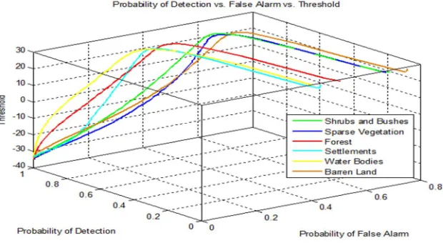
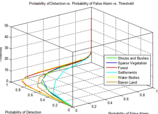
V. ROC GRAPHS

ROC curves/graphs are helpful for visualizing and organizing classifiers performance (Tom Fawcett et al., 2003). ROCs will remain unchanged with respect to the operating conditions (class skew and error costs). Conditions may change, the region of interest (ROI) may change, but the graph itself will remain constant (Tom Fawcett et al., 2003). ROCs are three-dimensional graphs among a threshold value, the probability of detection and false alarm. Three dimensional ROC graphs of our chosen classifiers are shown in figure 3 and 6. These graphs are drawn for finding optimum threshold points for achieving the best classification results. 3D ROC graphs are shown in Figure 3 and 6 for Maximum likelihood and Mahalanobis distance classifiers respectively. In order to find threshold, the optimal operating point is selected in detection vs false alarm curves are shown in figure 1 and 4, where the selected operating point has the maximum possible value of detection probability with minimum false alarm value.

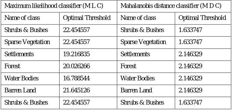
Table 2 Optimum threshold points of (MLC) and (MDC)

Maximum likelihood classifier (M L C) Mahalanobis distance classifier (M D C)

Name of class Optimal Threshold Name of class Optimal Threshold

Shrubs & Bushes 22.454557 Shrubs & Bushes 1.633747

Sparse Vegetation 22.454557 Sparse Vegetation 1.633747

Settlements 19.216835 Settlements 2.146329

Forest 20.026266 Forest 2.146329

Water Bodies 16.788544 Water Bodies 2.146329

Barren Land 21.645126 Barren Land 2.146329

Figure 1 RoC plot of MLC (detection vs. false alarm)

Generally, the optimum operating point is a point where 80 per cent detection lies along with least false alarm probability. To calculate a threshold value for target classification technique, the selected point is matched in the probability of detection vs threshold graphs which are shown in figure 2 and 5 respectively. This procedure is used to find the optimal threshold points, listed in table 2, for all the classes for both classification methods.

Figure 2 RoC graph of MLC (probability of detection vs. threshold)

Figure 3 3D RoC Graph of MLC

15 20 25 30

0 0.1 0.2 0.3 0.4 0.5 0.6 0.7 0.8 0.9 1

Probability of Detection vs. Threshold

Threshold

P

ro

b

a

b

ili

ty

o

f

D

e

te

c

ti

o

Figure 4 RoC Plot of MDC (detection vs. false Alarm)

Figure 5 RoC Graph of MDC (detection vs. threshold)

Figure 6 3D RoC Graph of MDC

0 0.1 0.2 0.3 0.4 0.5 0.6 0.7 0.8 0.9 1

0 0.1 0.2 0.3 0.4 0.5 0.6 0.7 0.8 0.9 1

Probability of Detection vs. False Alarm

Probability of False Alarm

P

ro

b

a

b

ilit

y

o

f

D

e

te

c

ti

o

n

VI. RESULTS AND DISCUSSIONS

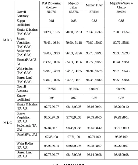
Results are achieved by pursuing a predefined process. Initially, we applied the chosen classification technique for each target class while considering 70 % training data. Optimal threshold values are found and selected from ROC curves shown above, for each classifier using threshold selection process explained in above section 5. Final classification on SPOT 5 image utilizing training ground truth data is applied to utilize optimal threshold values listed in table 2. The resultant classified image is saved and is used for obtaining end results. The confusion matrix is generated on testing data by considering the classified image as a reference to get the accuracy and kappa coefficient of the classification. Overall Accuracy (O A), Kappa Coefficient (Ka), User Accuracy (U A) and Producer Accuracies (PA) of the forest as well all other competing classes are displayed in table 4. As we can see from table 4, the MLC has achieved better results from that of Mahalanobis Distance classifier (M D C). OA and Ka values of M D C i.e, 85.97% and 0.81 are lower than those of MLC which are 97.65% and 0.96. Additionally, the producer accuracy for our main target class forest in M L C has higher value i.e. 97.35% in comparison with MDC with the producer accuracy of 83.72% as shown in Table 4.

Figure 7 original Spot 5 image

A. Post Processing

The obtained results are then further processed by applying the median, majority, sieve and clump filters. After applying these post-processing steps we achieved improved results as listed in Table 4. Forest producer accuracy is enhanced from 83.72% to 88.44% in M D C and it improved from 97.35% to 98.06% in case of M L C.

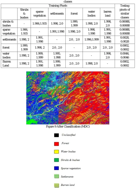
Table 3 Reparability factors (JM & TD) between any two classes of training data and between training and testing data of the same classes

Training Pixels Testing

pixels of similar classes Shrubs & bushes sparse

vegetation settlements forest

water bodies

barren land

shrubs &

bushes - 1.906,1.935 1.998, 2.0

1.999,

1.999 1.998, 2.0

1.998, 2.0 0.00088, 0.00088 sparse vegetation 1.906,

1.935 - 1.991,1.998 1.998, 2.0

1.998, 1.998 1.991, 1.998 0.00088, 0.00088

settlements 1.998, 2 1.991,

1.998 - 2.0 , 2.0 1.996,1.999

1.991, 1.998

0.0028, 0.0028

forest 1.999,

1.999 1.998, 2 2.0 , 2.0 - 2.0 , 2.0 2.0 , 2.0

0.0002, 0.0002 water

bodies 1.998, 2

1.999, 1.999

1.995,

1.998 2.0 , 2.0 -

1.998, 2.0

0.0046, 0.0046 Barren

Land 1.998, 2

1.991, 1.998

1.999,

1.999 2.0 , 2.0 1.998, 2.0 -

0.0002, 0.0002

Table 4 Classifiers’ results from confusion matrices before and after post-processing steps Post Processing

(Before)

Majority

Filter Median Filter

Majority+ Sieve + Clump

M D C

Overall Accuracy

85.97% 87.57% 87.53% 89.03%

Kappa-coefficient

0.81 0.83 0.83 0.85

Shrubs & bushes

(P A) (U A) 70.28 , 61.55 70.50 , 62.53 70.32 , 62.66 70.03 , 64.52

Sparse Vegetation (P A) (U A)

78.43 , 46.84 79.90 , 51.18 79.80 , 50.80 80.72 , 55.84

Settlements

(P A) (U A) 94.03 , 89.23 96.53 , 91.26 96.76 , 90.95 96.35 , 92.93

Forest (P A) (U

A) 83.72 , 98.34 85.83 , 98.56 85.77 , 98.58 88.44 , 98.51

Water bodies

(P A) (U A) 92.87 , 94.29 94.97 , 96.65 94.94 , 96.76 96.70 , 96.43

Barren Land

(P A) (U A) 93.07 , 98.36 94.37 , 98.61 94.36 , 98.66 95.53 , 98.54

M L C

Overall

Accuracy 97.65% 98.01% 98.01% 98.29%

Kappa-coefficient 0.96 0.97 0.97 0.97

Shrubs & bushes

(PA, UA) 97.77,99.07 98.16,99.07 98.16,99.04 98.29,99.10

Sparse Vegetation (PA, UA)

97.58,97.89 97.78,98.05 97.79,98.05 97.93,98.04

Settlements (PA,

UA) 97.84,98.61 98.45,98.56 98.45,98.42 98.81,98.59

Forest (PA, UA)

97.35,100 97.71,100 97.71,100 98.06,100

Water Bodies

(PA, UA) 98.92,99.94 99.06,99.97 99.03,98.97 99.20,99.97

Barren Land

(PA, UA) 97.75,99.97 98.15,99.98 98.14,99.98 98.45,99.98

VII. CONCLUSION

REFERENCES

[1] S. Wheeler and P. N. Misra, "Crop classification with Landsat multispectral scanner data II," Pattern Recognition, vol. 12, pp. 219-228, 1980.

[2] S. W. Buechel, W. R. Philipson, and W. D. Philpot, "The effects of a complex environment on crop separability with Landsat TM," Remote Sensing of Environment, vol. 27, pp. 261-271, 1989

[3] "Comparing Pixel-based Classifiers for Detecting Tobacco Crops in North-West Pakistan” by Aziz Ahmed, Muhammad Muaz, Manzoor Ali, Muhammad Yasir, Nasru Minallah, Shahbaz Khan, Department of Telecommunication Engineering, UET Peshawar, Pakistan

[4] S. Panigrahy and S. Sharma, "Mapping of crop rotation using multidate Indian Remote Sensing Satellite digital data," ISPRS Journal of Photogrammetry and Remote Sensing, vol. 52, pp. 85-91, 1997.

[5] D. Ehrlich, J. E. Estes, J. Scepan, and K. C. McGwire, "Crop area monitoring within an advanced ricultural information system," Geocarto International, vol. 9, pp. 31-42, 1994.

[6] C. Yang, J. H. Everitt, and D. Murden, "Evaluating high resolution SPOT 5 satellite imagery for crop identification," Computers and Electronics in Agriculture, vol. 75, pp. 347-354, 2011.

[7] P. Casals-Carrasco, S. Kubo, and B. B. Madhavan, "Application of spectral mixture analysis for terrain evaluation studies," International Journal of Remote Sensing, vol. 21, pp. 3039-3055, 2000.

[8] Roderick, M., R. C. G. Smith, and G. Ludwick. (1996). Calibrating long term AVHRR- derived NDVI imagery. Remote Sensing of Environment 58: 1-12. [9] J. A. Richards and J. Richards, Remote sensing digital image analysis vol. 3: Springer, 1999.

[10] H. Ibrahim, N. S. P. Kong, and T. F. Ng, "Simple adaptive median filter for the removal of impulse noise from highly corrupted images," IEEE Transactions on Consumer Electronics, vol. 54, pp. 1920-1927, 2008.

[11] Marconcini, M.; Fernandez-Prieto, D.; Buchholz, T., "Targeted Land-Cover Classification," in Geoscience and Remote Sensing, IEEE Transactions on, vol.52, no.7, pp.4173-4193, July 1 2014

[12] Weiqi Zhou, "An Object-Based Approach for Urban Land Cover Classification: Integrating LiDAR Height and Intensity Data," in Geoscience and Remote Sensing Letters, IEEE, vol.10, no.4, pp.928-931, July 2013

[13] Shiraishi, T.; Motohka, T.; Thapa, R.B.; Watanabe, M.; Shimada, M., "Comparative Assessment of Supervised Classifiers for Land Use–Land Cover Classification in a Tropical Region Using Time-Series PALSAR Mosaic Data," in Selected Topics in Applied Earth Observations and Remote Sensing, IEEE Journal of , vol.7, no.4, pp.1186-1199, April 2014.

[14] John A. Richards · Xiuping Jia, Canberra, Australia, January 2005, Remote Sensing Digital Image Analysis , Springer-Verlag Berlin Heidelberg 2006,4th Edition, p. 207