Computational Fluid Dynamics of Air Flow over the Exhaust Fan Wings with Different Curvature Angles

(1)

489 ©IJRASET: All Rights are Reserved

Computational Fluid Dynamics of Air Flow over

the Exhaust Fan Wings with Different Curvature

Angles

S. Maimum Siddiqi1, A Harsha Vardhan Reddy2, K Srinivas Yadavu3

1

Mechanical Engineering, GNITC, HYD 2

Mechanical Engineering Department, GNITC, HYD, 3

Mechanical Engineering, GNITC, HYD

Abstract: In this project, the transient Analysis (Dynamic analysis) is involved to find the deformation, stress per time of the exhaust fan of domestic air conditioning ducts because of change of speed axially. So this work deals with the speed and pressure changes.

In this, CFD process is involved to determine steam flow of the air around the fan wings. From the transient structural analysis, the deformation and stress as per the change of material properties and flow of air flow, vector direction of air, pressure and velocity as per the change of rpm’s can be defined.

Keywords:CATIA, ANYSIS, CFD

I. INTRODUCTION

Air conditioning (often referred to as AC, A/C, or air conditioners) is the process of removing heat and moisture from the interior of an occupied space, to improve the comfort of occupants. Air conditioning can be used in both domestic and commercial environments. This process is most commonly used to achieve a more comfortable interior environment, typically for humans or animals; however, air conditioning is also used to cool/dehumidify rooms filled with heat-producing electronic devices, such as computer servers, power amplifiers, and even to display and store artwork.

Air conditioners often use a fan to distribute the conditioned air to an occupied space such as a building or a car to improve thermal comfort and indoor air quality. Electric refrigerant-based AC units range from small units that can cool a small bedroom, which can be carried by a single adult, to massive units installed on the roof of office towers that can cool an entire building. The cooling is typically achieved through a refrigeration cycle, but sometimes evaporation or free cooling is used. Air conditioning systems can also be made based on desiccants (chemicals which remove moisture from the air) and subterraneous pipes that can distribute the heated refrigerant to the ground for cooling.

In the most general sense, air conditioning can refer to any form of technology that modifies the condition of air (heating, cooling, (de-)humidification, cleaning, ventilation, or air movement). In common usage, though, "air conditioning" refers to systems which cool air. In construction, a complete system of heating, ventilation, and air conditioning is referred to as heating, ventilation, and air conditioning.

II. LITERATURE REVIEW

As all of us understand that the purpose of ventilation is to reduce or dilute the indoor contaminants, the experienced engineers should determine how much air is necessary to dilute and reduce the contaminants to a desired level. The existence of ventilation and indoor air quality can be traced back to 17th century. However, concerns about the bad air go back much farther than that. One of the earliest reasons to implement the idea of ventilation is to ventilate

(2)

490 ©IJRASET: All Rights are Reserved

III. PART MODELING A. Project Objective

In this chapter, we will be able to:

1) Understand the design modeller workshop

2) Draw sketches

3) Convert sketches into 3d models

4) Understand views of the model in 3d space

5) Apply constraints and relations

Geometry

Fig 1 Geometry of Exhaust Fan Wings

B. Introduction To Ansys Workbench

In ansys workbench this are the list of analysis can be determined:

1) Modal analysis

2) Static structural analysis

3) Transient structural analysis

4) Steady state thermal analysis

5) Transient thermal analysis

6) Fluid flow (CFD) etc.

C. Introduction To Modal Analysis

The modal analysis is used to calculate the vibration characteristics such as natural frequency and mode shape (deformed shapes) of a structure or a machine component. The output of the modal analysis can be further used as input for the harmonic and transient analyses.

For example, a cantilever beam, attached to a system vibrating at a certain frequency. It is important for the designer to ﬁnd out

whether the beam will sustain the vibrations induced by the machine to which it is connected.

When the cantilever vibrates, various shapes are attained at certain frequencies. The shape of the component corresponding to a frequency is known as mode shape. The mode shape is a graphical representation of the deformation attained due to vibration. The main aim of the modal analysis is to ﬁnd whether the natural frequency of the component is closer to the vibrations induced in the component. In this example, with this cantilever, the maximum number of modes found is six. Through display the various mode shapes of ﬁrst, second, 3rd, and 4th modes, respectively.

(3)

491 ©IJRASET: All Rights are Reserved

time/frequency-based loads. If the stress/strain/displacement response is less than the permissible limit, the component will not be required to strengthen or redesign.

1) Performing the Modal Analysis: The Modal analysis is performed to ﬁnd out the natural frequencies of a model. You can ﬁnd

out more than one natural frequency of a model depending upon the degrees of freedom available. The following steps are involved to perform a Modal analysis:

a) Set the analysis preference.

b) Create or import the geometry into ANSYS Workbench.

c) Deﬁne element attributes (element types, real constants, and material properties). d) Deﬁne meshing attributes.

e) Generate a mesh for the model.

f) Specify the analysis type, analysis options, and apply loads.

g) Obtain the solution.

h) Review the results.

i) Most of these steps have already been discussed in previous chapters.

2) Adding Modal Analysis System to ANSYS Workbench: To perform a Modal analysis in ANSYS Workbench, you need to add the Modal analysis system from the Analysis Systems toolbox in the Toolbox window to the Project Schematic window,

3) Starting the Mechanical Window: To start the analysis, double-click on the Model cell of the Modal analysis system to display the Mechanical window. The components of the Mechanical window displayed by using the Model cell of the Modal analysis system are similar to the components of the Mechanical window displayed by using the Static Structural analysis system.

Fig. 2The Mechanical window with the Modal node displayed in the Tree Outline

In the Mechanical window, you can set the number of modes or natural frequencies you need To ﬁnd shows the Tree Outline of the Mechanical window.

(4)

492 ©IJRASET: All Rights are Reserved

5) Plotting the Deformed Shape (mode shape): You can plot the mode shape (deformed shape) at each mode. However, before plotting the deformed shape need, you need to specify the mode in the Graph window. To create the mode shapes, select the Solution node in the Tree Outline; the Graph and Tabular Data windows will be displayed in the Graphics screen. Now right click in the Graph window to display a shortcut menu and then choose Select All from it. Right-click again in the Graph window and then choose the Create Mode Shape Results option from the shortcut menu; the modes are added under the Modal node. Based on the number speciﬁed in the Max Modes to Find edit box, the numbers of modes are created with the names

Total Deformation, Total Deformation 2 . . . Total Deformation 6. Select the required mode from the Solution node to visualize the corresponding mode shape in the Graphics screen.

a) Step 1: Starting a New Project and Creating the Model

The first step is to start a new project in the Workbench window.

i) Start ANSYS Workbench.

ii) Choose the Save button from the Standard toolbar; the Save As modal analysis on fan clutch.

iii) Double-click on modal in the Toolbox window; the modal analysis system is added in the Project Schematic window.

iv) Now we can see the cell of modal which having the engineering data, geometry selection, modal, setup, solution and results as mention in chapter 4.

v) In the ANSYS Workbench dialog box, set the unit to millimeter.

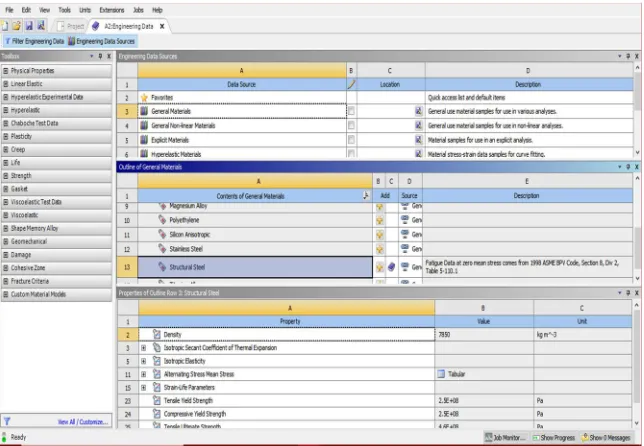
b) Step 2: Adding the Material to the Engineering Data

After adding the modal analysis into project schematics. We have chosen the materials for the modal.

i) First go the static structural analysis on project schematic. Then Double-click on the Engineering Data cell. It will make a link to the Engineering Data workspace is displayed in the Workbench window.

ii) Choose the Engineering Data Sources toggle button from the Standard toolbar; the Engineering Data Sources window is added to the Engineering Data workspace. In the Engineering Data Sources window, select the General Materials library to display the Outline of General Materials window.

iii) In the Outline of General Materials window, choose the plus symbol corresponding to Aluminum Alloy, etc. material; the material is added to the Engineering Data in the Outline window of the Engineering Data workspace. Again, choose the Engineering Data Sources toggle button from the Standard toolbar to switch to the default view of Engineering Data workspace. Choose the Return to Project button from the Standard toolbar to display at the top the Project Schematic window.

Fig. 3 Specifying a Material

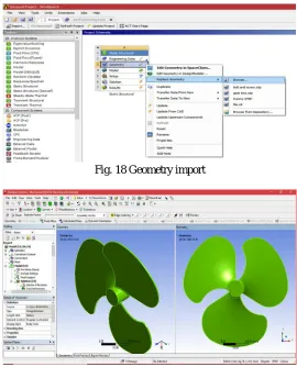
c) Step 3: Geometry creation or import geometry

For analysis we required the geometry to analysis. As per the chapter 5, we need to design or import the geometry. In ansys software we have designer module and space clam software which allows redesigning or creating the geometry in ansys software. Similarly, we can also import the geometry, by using any one of the designing or cad (computer aided design and drafting) software to create the model. Later the modal should be converted into step file (standard exchange programming file).

(5)

493 ©IJRASET: All Rights are Reserved

Fig 4 Geometry import

Modal 1 at wing 26°

(6)

494 ©IJRASET: All Rights are Reserved

d) Step 4: Generating the Mesh

After the model is created in the Design Modeler window, you need to generate the mesh for the model in the Mechanical window.

i) Again go to the modal analysis – select the model cell in it, double-click on the Model cell in the modal analysis system; we will enter Mechanical window is displayed.

ii) In model cell we here see the outline of the project and below that detail view will be present. In middle we can see the component in graphical. On right side of the window, graph and table data will be located.

iii) Now go to the meshing and right click- select generate mesh. Select Mesh in the Tree Outline to display the Details of "Mesh" window, we can the size of meshing process if the geometry conditions are required. In general, meshing sizes don’t not be less 5 mm for rigid body and max is 15mm.

iv) In the Details of "Mesh" window, expand the Sizing node, if it is not already expanded. Also, notice that Default is displayed in the Element Size edit box.

Fig. 7 Mesh generated with default mesh controls

Expand the Statistics node in the Details of "Mesh" window to display the total number of elements created. On doing so, you will find that the total number of elements.

e) Step 5: Specifying the Boundary Conditions

After you mesh the model, it is required to specify the boundary and loading conditions.

i) In the Mechanical window, select the modal analysis from the Tree Outline; the Details of “modal” window is displayed along with the Environment contextual toolbar.

ii) Choose the Fixed Support tool from the Supports drop-down in the Environment contextual toolbar; Fixed Support is added under the Static Structural node. Also, the Details of “ fixed support ” window is displayed

iii) Click on the Geometry selection box to display the Apply and Cancel buttons

iv) Choose the Face tool or body from the Select toolbar to enable selection of faces.

(7)

495 ©IJRASET: All Rights are Reserved

v) Select faces on the model. Next, choose the Apply button in the Geometry selection box; the selected faces turn purple indicating that Fixed support is applied

vi) Later go analysis setting then specify the maximum of mode shape. Change or specify the value in between 1to 999999 modes shapes.

Fig. 9 The violet face of the model displaying the Fixed supports

f) Step 6: Solving the FE Model and Analyzing the Results

After the boundary and conditions are speciﬁed for the model, you need to solve the analysis. After solving, you will get the Total and Directional Deformations due to the given condition. Select the Solution node in the Tree Outline; the Solution contextual toolbar is displayed. Also, the Details of “Solution” window is displayed.

i) Choose the Total tool from the Deformation drop-down of the Solution contextual toolbar; Total Deformation is added under the Solution node.

Fig 10 The maximum and minimum values of Total Deformation can also be obtained from the Legend displaying the color bands in the Graphics screen

10. Select all other parameters from the Solution node; the respective view is displayed in the Graphics screen. The table given next lists all the results obtained from the analysis. Show the corresponding graphical representation of values obtained.

(8)

496 ©IJRASET: All Rights are Reserved

Fig. 11 Total deformation at 1st 2nd 3rd and 4th modes

Fig 12 Total deformation at 5th 6th 7th and 8th modes

Table 1 Values of Total Deformation, Frequency for 26°

Results for al alloy for modal 1 (angle 25°)

Fig. 13 Total deformation at 1st 2nd 3rd and 4th modes

S.No Deformation Frequency Vibrations

Mm Hz Mm*Mm/

Hz

1 0.91818 92.906 0.008399

2 0.93249 97.608 0.004987

3 0.92465 100.33 0.004911

4 1.5345 258.68 0.003492

5 1.5409 260.83 0.00455

6 1.5199 264.35 0.005374

7 1.1682 442.18 0.003167

(9)

497 ©IJRASET: All Rights are Reserved

Fig. 14 Total deformation at 5th 6th 7th and 8th modes

Table. 15 Values of Total Deformation, Frequency for 25°

Results for al alloy for modal 1 (angle 24°)

Fig. 16 Total deformation at 1st 2nd 3rd and 4th modes Fig.17 Total deformation at 5th 6th 7th and 8th modes

S.No Deformation Frequency Vibrations

Mm Hz Mm*Mm/Hz

1 0.91981 95.303 0.00887748

2 0.9271 97.587 0.00880767

3 0.90789 98.159 0.00839724

4 1.5248 241.36 0.00963298

5 1.5334 242.37 0.00970135

6 1.5297 242.83 0.0096363

7 1.1433 455.66 0.00286866

(10)

498 ©IJRASET: All Rights are Reserved

S.No Deformation Frequency Vibrations

Mm Hz Mm*Mm/Hz

1 0.89754 88.07 0.00914702

2 0.90693 91.268 0.009012162

3 0.90575 95.613 0.008580246

4 1.5545 209.38 0.011541075

5 1.5611 211.02 0.011548826

6 1.5155 215.01 0.010682016

7 1.1321 406.35 0.003154055

[image:10.612.183.449.91.453.2]

8 1.1319 419.06 0.003057313

Table. 2 Values of Total Deformation, Frequency for 24°

Fig. 16 Random vibrations Graph

IV. INTRODUCTION TO STATIC STRUCTURAL ANALYSIS A. Introduction

In this project, we imported the geometry of the component show the dimensions for the component with respect to the load applications. The material to be applied on the model is Stainless Steel. Next, you will run the analysis under two conditions and evaluate the Total Deformation, Directional Deformation, Equivalent Stress, Maximum Principal Stress, and Minimum Principal Stress.

The Static Structural analysis is one of the important analyses in ANSYS Workbench. It is available as Static Structural analysis system under the Analysis System toolbox in the Toolbox window, this system analyses the structural components for displacements (deformation), stresses, strains, and forces under different loading conditions. The loads in this analysis system are assumed not to have damping characteristics (time dependent). Steady loading and damping conditions are assumed in this type of analysis system.

To start a new Static Structural analysis system, double-click on Static Structural in the Analysis Systems toolbox in the Toolbox window; the Static Structural analysis system will be added to the Project Schematic window.

(11)

499 ©IJRASET: All Rights are Reserved

B. Project Overview

Analysis on static structural analysis

1) Start a new project and create the model.

2) Generate the mesh.

3) Set the boundary and loading _conditions.

4) Solve the model.

5) Duplicate the existing analysis system.

6) Interpret results.

7) Save the project.

a) Step 1: Starting a New Project and Creating the Model

i) Start ANSYS Workbench.

ii) Choose the Save button from the Standard toolbar; the Save As static structural analysis on fan

iii) Double-click on Static Structural in the Toolbox window; the Static Structural analysis system is added in the Project Schematic window.

iv) Now we can see the cell of static structural analysis which having the engineering data, geometry selection, modal, setup, solution and results as mention in chapter 4.

v) In the ANSYS Workbench dialog box, set the unit to millimeter.

b) Step 2: Adding the Material to the Engineering Data

After adding the static structural analysis into project schematics. We have chosen the materials for the modal.

i) First go the static structural analysis on project schematic. Then Double-click on the Engineering Data cell. It will make a link to the Engineering Data workspace is displayed in the Workbench window.

ii) Choose the Engineering Data Sources toggle button from the Standard toolbar; the Engineering Data Sources window is added to the Engineering Data workspace.

iii) In the Engineering Data Sources window, select the General Materials library to display the Outline of General Materials window.

iv) In the Outline of General Materials window, choose the plus symbol corresponding to Aluminum Alloy, etc material; the material is added to the Engineering Data in the Outline window of the Engineering Data workspace.

v) Again, choose the Engineering Data Sources toggle button from the Standard toolbar to switch to the default view of Engineering Data workspace.

[image:11.612.146.468.495.718.2]

Choose the Return to Project button from the Standard toolbar to display at the top the Project Schematic window.

(12)

500 ©IJRASET: All Rights are Reserved

7.3.2 Aluminum Alloy

Aluminum Alloy > Constants

Density 2.77e-006 kg mm^-3

Isotropic Secant Coefficient of Thermal Expansion 2.3e-005 C^-1

Specific Heat 8.75e+005 mJ kg^-1 C^-1

i) Aluminum Alloy > Compressive Yield Strength Compressive Yield Strength MPa

280

Aluminum Alloy > Tensile Yield Strength Tensile Yield Strength MPa

280

Aluminum Alloy > Tensile Ultimate Strength Tensile Ultimate Strength MPa

310

Aluminum Alloy > Isotropic Secant Coefficient of Thermal Expansion Zero-Thermal-Strain Reference Temperature C

22

Aluminum Alloy > Isotropic Thermal Conductivity Thermal Conductivity W mm^-1 C^-1 Temperature C

0.114 -100

0.144 0

0.165 100

0.175 200

Aluminum Alloy > Isotropic Resistivity Resistivity ohm mm Temperature C

2.43e-005 0

2.67e-005 20

3.63e-005 100

Aluminum Alloy > Isotropic Elasticity Temperature C Young's Modulus

MPa

Poisson's Ratio Bulk Modulus MPa

Shear Modulus MPa

71000 0.33 69608 26692

c) Step 3: Geometry creation or import geometry

For analysis we required the geometry to analysis. As per the chapter 5, we need to design or import the geometry.

In Ansys software we have designer module and space clam software which allows redesigning or creating the geometry in ansys software. Similarly we can also import the geometry, by using any one of the designing or cad (computer aided design and drafting) software to create the model. Later the modal should be converted into step file (standard exchange programming file).

(13)

501

[image:13.612.170.440.74.408.2]

©IJRASET: All Rights are Reserved

Fig. 18 Geometry import

Fig. 18 Modal in static structuralanalysis

d) Step 4: Generating the Mesh

i) Again go to the static structural analysis – select the model cell in it, double-click on the Model cell in the static structural analysis system; we will enter Mechanical window is displayed.

ii) In model cell we here see the outline of the project and below that detail view will be present. In middle we can see the component in graphical. On right side of the window, graph and table data will be located.

iii) Now go to the meshing and right click- select generate mesh. Select Mesh in the Tree Outline to display the Details of "Mesh" window, we can the size of meshing process if the geometry conditions are required. In general, meshing sizes don’t not be less 5 mm for rigid body and max is 15mm.

iv) In the Details of "Mesh" window, expand the Sizing node, if it is not already expanded. Also, notice that Default is displayed in the Element Size edit box.

(14)

502 ©IJRASET: All Rights are Reserved

v) Expand the Statistics node in the Details of "Mesh" window to display the total number of elements created. On doing so, you will find that the total number of elements.

e) Step 5: Specifying the Boundary Conditions: After you mesh the model, it is required to specify the boundary and loading conditions.

i) In the Mechanical window, select the Static Structural node from the Tree Outline; the Details of “Static Structural” window is displayed along with the Environment contextual toolbar.

ii) Choose the Fixed Support tool from the Supports drop-down in the Environment contextual toolbar; Fixed Support is added under the Static Structural node. Also, the Details of “ Static Structural” window is displayed

iii) Click on the Geometry selection box to display the Apply and Cancel buttons

iv) Choose the Face tool or body from the Select toolbar to enable selection of faces.

v) Select faces on the model. Next, choose the Apply button in the Geometry selection box; the selected faces turn purple indicating that Fixed support is applied

vi) Choose the Force tool from the Loads drop-down in the Environment contextual toolbar; Force is added under the Static Structural node in the Tree Outline. Also, the Details of “Force” window is displayed

vii) Click on the Geometry selection box to display the Apply and Cancel buttons, if they are not already displayed.

viii) Next, select the face on the right of the model, as shown in Figure.

ix) Choose the Apply button from the Geometry selection box; the face turns red indicating that the Force load is applied.

x) In the Details of “Force” window, expand the Deﬁnition node, if it is not already expanded. xi) Select Vector from the Deﬁne By drop-down list, if it is not already selected.

xii) In the Details of “Force” window, click on the right arrow next to the Magnitude edit Box; a ﬂy-out is displayed.

xiii) In the Magnitude edit box, enter number. Click on the Direction selection box to display the Apply and Cancel buttons. As the application of force under consideration is vertically downward, you need to Deﬁne the direction by selecting edges for the

force vector.

xiv) Next, choose the Apply button from the Direction selection box; a downward force is speciﬁed for the analysis. After you have

selected the edge for specifying the direction, you can ﬂip the direction xv) Speciﬁed by choosing the Flip button available in the Graphics screen.

Fig 20 The violet and red color face of the model displaying the fixed support and pressure

f) Step 6: Solving the FE Model and Analyzing the Results

After the boundary and load conditions are speciﬁed for the model, you need to solve the analysis. After solving, you will get the Total and Directional Deformations due to the given condition. Also, you will get Equivalent Stress, Maximum Principal, and Minimum Principal Stresses.

i) Select the Solution node in the Tree Outline; the Solution contextual toolbar is displayed. Also, the Details of “Solution” window is displayed.

(15)

503 ©IJRASET: All Rights are Reserved

Fig. 20 The maximum and minimum values of Total Deformation can also be obtained from the Legend displaying the color bands in the Graphics screen

iii) Select all other parameters from the Solution node; the respective view is displayed in the Graphics screen. The table given next lists all the results obtained from the analysis. Show the corresponding graphical representation of values obtained.

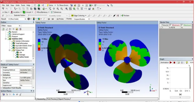
g) Step 6: Color contours displaying the result: Results for aluminum alloy; if fan is made up of aluminum alloy

i) Modal at angle 26°

Fig. 21Total deformation of the 26° fan

[image:15.612.31.496.266.712.2]

ii) Modal at angle 25°

(16)

504 ©IJRASET: All Rights are Reserved

iii) Modal at angle 24°

Fig. 23Total deformation of the fan 24° and its selection view

The value that is displayed next to each color is the Total Deformation in the region which Is depicted by that particular color in the model. The blue color in the model represents the lowest value of the Total Deformation, whereas the red color denotes the maximum value of The Total Deformation.

[image:16.612.127.484.307.510.2]

iv) Modal at angle 26°

Fig 24 Equivalent strain of the 26°fan

v) Modal at angle 25°

(17)

505 ©IJRASET: All Rights are Reserved

vi) Modal at angle 24°

Fig. 26 Equivalent strain of the fan 24° and its selection view

The value that is displayed next to each color is the equivalent strain in the region which Is depicted by that particular color in the model. The blue color in the model represents the lowest value of the equivalent strain, whereas the red color denotes the maximum value of the equivalent strain.

vii) Modal at angle 26°

Fig. 27 Equivalent stress of the 26° fan

viii) Modal at angle 25°

(18)

506 ©IJRASET: All Rights are Reserved

ix) Modal at angle 24°

Fig.29 Equivalent stress of the fan and its selection view

The value that is displayed next to each color is the equivalent stress in the region which is depicted by that particular color in the model. The blue color in the model represents the lowest value of the equivalent stress, whereas the red color denotes the maximum value of the equivalent stress.

Fatigue tools:

After the selection stress, strain and deformation of the modal, the effect of friction is more important because of the body is in dynamics. In general in all rotating and siding assemble gets effects by the frictional loads and pressure due to another body due to the dynamics it may damage, life change and also we can assure safety factor

Go to solution, right click over it then select the Fatigue tools. In contact tools- right click and select damage, life change and also we can assure safety factor (if) can be selected to find the results.

x) Modal at angle 26°

Fig. 30 Life of vertical 26°

xi) Modal at angle 25°

(19)

507 ©IJRASET: All Rights are Reserved

xii) Modal at angle 24°

Fig. 32 Life of vertical

The value that is displayed next to each color is the life in the region which is depicted by that particular color in the model. The blue color in the model represents the lowest value of the life, whereas the red color denotes the maximum value of the life.

xiii) Modal at angle 26°

Fig 33 Damages of vertical 26°

xiv) Modal at angle 25°

(20)

508 ©IJRASET: All Rights are Reserved

xv) Modal at angle 24°

Fig. 35 Damages of vertical

The value that is displayed next to each color is the damages in the region which Is depicted by that particular color in the model. The blue color in the model represents the lowest value of the damages, whereas the red color denotes the maximum value of the damages.

[image:20.612.147.467.327.495.2]

xvi) Modal at angle 26°

Fig. 36 Safety factor of vertical 26°

xvii) Modal at angle 25°

(21)

509 ©IJRASET: All Rights are Reserved

[image:21.612.183.431.91.251.2]

xviii) Modal at angle 24°

Fig 38 Safety factor of vertical

(22)

510

[image:22.612.120.496.90.175.2]

©IJRASET: All Rights are Reserved

Table 3 values of static structural Total deformation, Stress, Strain, Life, Damage, Safety Factor

V. TRANSIENT STRUCTURAL (Dynamic) ANALYSIS

A. Introduction

In this project, we imported the geometry of the component show the dimensions for the component with respect to the load applications. The material to be applied on the model is Stainless Steel. Next, you will run the analysis under two conditions and evaluate the Total Deformation, Directional Deformation, Equivalent Stress, Maximum Principal Stress, and Minimum Principal Stress.

The transient structural (dynamic) analysis is one of the important analyses in ANSYS Workbench. It is available as transient structural (dynamic) analysis system under the Analysis System toolbox in the Toolbox window, this system analyses the structural components for displacements (deformation), stresses, strains, and forces under different loading conditions with respect to time or step. The loads in this analysis system are assumed not to have damping characteristics (time dependent). Steady loading and damping conditions are assumed in this type of analysis system.

To start a new transient structural (dynamic) analysis system, double-click on transient structural (dynamic) in the Analysis Systems toolbox in the Toolbox window; the transient structural (dynamic) analysis system will be added to the Project Schematic window. To start an analysis, first you need to specify the geometry on which the analysis is to be done. To do so, you can import the geometry from an external CAD package, or you can create the geometry in the ANSYS's Design Modeler software. After the model is specified for an analysis, you need to double-click on the Model cell of the transient structural (dynamic) analysis system to open the Mechanical window. In this window, you can specify the parameters and run the analysis.

As discussed in previous chapters, analysis can be carried out in three major steps: pre-processing, solution, and post-processing. The tools required to carry out these steps are discussed next.

1) Step 1: Starting a New Project and Creating the Model

a) Start ANSYS Workbench.

b) Choose the Save button from the Standard toolbar; the Save As static structural analysis on vertical turbine

c) Double-click on Static Structural in the Toolbox window; the Static Structural analysis system is added in the Project Schematic window.

d) Now we can see the cell of static structural analysis which having the engineering data, geometry selection, modal, setup, solution and results as mention in chapter 4.

e) In the ANSYS Workbench dialog box, set the unit to millimeter.

2) Step 2: Adding the Material to the Engineering Data

After adding the structural analysis into project schematics. We have chosen the materials for the modal.

a) First go the static structural analysis on project schematic. Then Double-click on the Engineering Data cell. It will make a link to the Engineering Data workspace is displayed in the Workbench window.

b) Choose the Engineering Data Sources toggle button from the Standard toolbar; the Engineering Data Sources window is added to the Engineering Data workspace.

c) In the Engineering Data Sources window, select the General Materials library to display the Outline of General Materials window.

d) In the Outline of General Materials window, choose the plus symbol corresponding to Aluminum Alloy, etc. material; the material is added to the Engineering Data in the Outline window of the Engineering Data workspace.

e) Again, choose the Engineering Data Sources toggle button from the Standard toolbar to switch to the default view of Engineering Data workspace.

Choose the Return to Project button from the Standard toolbar to display at the top the Project Schematic window.

Angle 26 39.04 0.017663 1084.2 853238.1 201.435 1

Angle 25 37.853 0.016967 1195.6 307095.5 684.661 1

Angle 24 43.804 0.018044 12319 2601540 853.368 1

Strain Mm/Mm

Stres s

Mpa Life Damage Safety Factor

(23)

511 ©IJRASET: All Rights are Reserved

3) Step 3: Geometry creation or import geometry.

For analysis we required the geometry to analysis. As per the chapter 5, we need to design or import the geometry.

In ansys software we have designer module and space clam software which allows redesigning or creating the geometry in ansys software. Similarly, we can also import the geometry, by using any one of the designing or cad (computer aided design and drafting) software to create the model. Later the modal should be converted into step file (standard exchange programming file).

[image:23.612.177.434.159.297.2]

To this go geometry cell and right click over it the select browser. Then go the browser file and select the. STEP file to import.

Fig 39 Modal in transient structural analysis

4) Step 4: Generating the Mesh

a) Again go to the static structural analysis – select the model cell in it, double-click on the Model cell in the static structural analysis system; we will enter Mechanical window is displayed.

b) In model cell we here see the outline of the project and below that detail view will be present. In middle we can see the component in graphical. On right side of the window, graph and table data will be located.

c) Now go to the meshing and right click- select generate mesh. Select Mesh in the Tree Outline to display the Details of "Mesh" window, we can the size of meshing process if the geometry conditions are required. In general, meshing sizes don’t not be less 5 mm for rigid body and max is 15mm.

d) In the Details of "Mesh" window, expand the Sizing node, if it is not already expanded. Also, notice that Default is displayed in the Element Size edit box.

Fig. 40 Mesh generated with default mesh controls

Expand the Statistics node in the Details of "Mesh" window to display the total number of elements created. On doing so, you will find that the total number of elements.

5) Step 5: Specify the frictional contacts

After the geometry selection we will get defaults contact tools (pre-selection contact surfaces as a bonding together). In contact region change the type to frictional and specify the boundary of frictional stiff will be 0.1 and 0.2 if necessary.

[image:23.612.182.429.473.621.2]

(24)

512 ©IJRASET: All Rights are Reserved

6) Step 6: Specifying the Boundary Conditions

After you mesh the model, it is required to specify the boundary and loading conditions.

a) In the Mechanical window, select the Static Structural node from the Tree Outline; the Details of “Static Structural” window is displayed along with the Environment contextual toolbar.

b) Choose the Fixed Support tool from the Supports drop-down in the Environment contextual toolbar; Fixed Support is added under the Static Structural node. Also, the Details of “transient structural analysis” window is displayed if needed

c) Click on the Geometry selection box to display the Apply and Cancel buttons

d) Choose the Face tool or body from the Select toolbar to enable selection of faces.

e) Select faces on the model. Next, choose the Apply button in the Geometry selection box; the selected faces turn purple indicating that Fixed support is applied

f) Choose the remote displacement tool from the Loads drop-down in the Environment contextual toolbar; remote displacement is added under the transient Structural node in the Tree Outline. Also, the Details of “remote displacement” window is displayed

g) Click on the Geometry selection box to display the Apply and Cancel buttons, if they are not already displayed.

h) Next, select the face on the right of the model, as shown in Figures.

i) Choose the Apply button from the Geometry selection box; the face turns yellow indicating that the displacement load is applied.

j) In the Details of “remote displacement” window, expand the Deﬁnition node, if it is not already expanded.

k) Select Vector from the Deﬁne By drop-down list, if it is not already selected. Only z axis rotation is free or making a rotation (rpm) will be mention.

l) In the Details of “remote displacement” window, click on the right arrow next to the Magnitude edit Box; a ﬂy-out is displayed.

m) In the Magnitude edit box, enter number.

After you have selected the edge for specifying the direction, you can ﬂip the direction. Speciﬁed by choosing the Flip button

available in the Graphics screen.

Fig 41 The yellow color face of the model displaying the remote displacement support

7) Step 7: Solving the FE Model and Analyzing the Results

After the boundary and load conditions are speciﬁed for the model, you need to solve the analysis. After solving, you will get the Total and Directional Deformations due to the given condition. Also, you will get Equivalent Stress, Maximum Principal, and Minimum Principal Stresses.

a) Select the Solution node in the Tree Outline; the Solution contextual toolbar is displayed. Also, the Details of “Solution” window is displayed.

b) Choose the Total tool from the Deformation drop-down of the Solution contextual toolbar; Total Deformation is added under the Solution node.

(25)

8) Step 8: Color contours displaying the result

Results for al alloy; if fan is made up of al alloy,

a) Modal at angle 26°

Fign 42 Total deformation of 26° fan

[image:25.612.171.442.116.248.2]

b) Modal at angle 25°

Fig 43 Total deformation of 25° fan

c) Modal at angle 24°

Fig 44 Total deformation of 24°fan

[image:25.612.168.445.289.430.2]

(26)

[image:26.612.157.455.90.244.2]

d) Modal at angle 26°

Fig. 45 Equivalent strain of 26° fan

[image:26.612.160.457.288.453.2]

e) Modal at angle 25°

f) Modal at angle 24°

[image:26.612.153.460.492.688.2]

(27)

[image:27.612.149.463.90.252.2]

g) Modal at angle 26°

Fig. 48 Equivalent stress of 26° fan

[image:27.612.120.481.294.460.2]

h) Modal at angle 25°

Fig .49 Equivalent stress of 25° fan

i) Modal at angle 24°

Fig 50 Equivalent stress of 24° fan

[image:27.612.139.474.505.678.2]

(28)

516

[image:28.612.71.552.89.337.2]

Table. 8.1 Values of Transient Structural Total Deformation, eq. Stress, eq. Strain

VI. COMPUTATIONAL FLUID DYNAMICS

Computational Fluid Dynamics (CFD) is a computer-based tool for simulating the behavior of systems involving fluid flow, heat transfer, and other related physical processes. It works by solving the equations of fluid flow (in a special form) over a region of interest, with specified (known) conditions on the boundary of that region.

Computers have been used to solve fluid flow problems for many years. Numerous programs have been written to solve either specific problems, or specific classes of problems. From the mid-1970s, the complex mathematics required to generalize the algorithms began to be understood, and general purpose CFD solvers were developed. These began to appear in the early 1980s and required what were then very powerful computers, as well as an in-depth knowledge of fluid dynamics, and large amounts of time to set up simulations. Consequently, CFD was a tool used almost exclusively in research.

Recent advances in computing power, together with powerful graphics and interactive 3D manipulation of models, have made the process of creating a CFD model and analyzing results much less labor intensive, reducing time and, hence, cost. Advanced solvers contain algorithms that enable robust solutions of the flow field in a reasonable time.

As a result of these factors, Computational Fluid Dynamics is now an established industrial design tool, helping to reduce design time scales and improve processes throughout the engineering world. CFD provides a cost-effective and accurate alternative to scale model testing, with variations on the simulation being performed quickly, offering obvious advantages.

A. Uses of CFD

CFD is used by engineers and scientists in a wide range of fields. Typical applications include:

1) Process Industry: Mixing vessels, chemical reactors

2) Building Services: Ventilation of buildings, such as atriums

3) Health And Safety: Investigating the effects of fire and smoke

4) Motor Industry: Combustion modeling, car aerodynamics

5) Electronics: Heat transfer within and around circuit boards

6) Environmental: Dispersion of pollutants in air or water

7) Power And Energy: Optimization of combustion processes

8) Medical: Blood flow through grafted blood vessels

B. Modal Imported

1) Go to Ansys software and select import from top left corner and Browser to step file

(29)

C. Meshing

1) After importing go the analysis setting and select Ansys fluid flow and drag and leave on project schematic window as shown in figure

[image:29.612.185.426.132.264.2]

2) Later go to meshing and double over it. Now we can enter into the analysis fluid flow mechanical fluent window

Fig. 9.2 Modal in Fluid Flow Fluent

Now go to the meshing under the tree outline. Then specify the mesh size should be fewer than 512 k elements.

After the mesh was generated, go to the selection, then the front of the rectangle and right over it then selects named selection. Under the named selected it as “inlet”. Again, go to the selection, and then the back of the rectangle and right over it then selects named selection. Under the named selected it as “outlet”.

Fig. 9.3 After the Name Selecting, Go to File and Select the Close Meshing

D. Fluent Fluid Flow Process

After the meshing, go to file and select meshing close. Then we will come back to the project schematic. In project schematics under the fluid flow fluent double click on the setup. Then we get fluent launcher (setting editing only). Then select parallel under it –click ok.

1) Step 1: under the fluent flow fluent go to the tree and select or double click on the general. In middle general properties will be

modify and select the transient. Then click on unit to change the temperature k to c. Then click ok.

2) Step 2: Model Type: After the general setting, double click on the models. In model settings, make energy –on, so that temperature can be applied over the heat exchangers. After that, double click on the viscous model. In viscous model go to the model and select the k-epsilon (2 equations.). In k- epsilon model, select the rng. In rng, select swirls dominated flow and under near wall treatment select scalable wall function. Then select ok to confirm.

3) Step 3: Material Selection: After that, model setting. Double click on the materials under the material task page, double click on the fluid. In fluid create / edit, select the order material by name and select the fluent data base. In fluid database materials, select the water –liquid as a material for the inlet fluid. And similarly select material under create or edit, change the fluid to solid and select the material as aluminum alloy.

[image:29.612.190.435.336.455.2]

(30)

5) Step 5: Mesh Interface: The interface helps to transfer the temperature between the body and liquid as same as contact region in transient thermal analysis. Go to mesh interface and double click over it. Under the mesh interface – select edit- and select interface 1 and 2 is coupled wall then select ok to confirm.

6) Step 6: Boundary Conditions: Now go to the boundary condition and double click over it. In boundary condition select the inlet and specify the boundary conditions are velocity 2 m/s (120m/min)

7) Step 7: Solution- Calculation Activities: Go to tree outline double on the calculation activities under solution. In calculation activities select automatic export- create-file type – cfd-post –select all quantities then click ok.

8) Step 8: Results Calculation: Double click on the run calculation- then specify the time steps 0.1 sec and number of time steps should be 20 then go to max iterations/ time step = 20. (0.1*20=2 sec)

[image:30.612.172.444.239.354.2]

Go to the run calculation and double click over it. Then click on calculation to run simulation process. The process will completed upon 10 or (sec)*25 or (iteration)*10 or (time steps)= 2500 iteration as shown in below.

Fig.51 Run Calculation Activities- Iterations

E. Results

Three reference line meshing for flow direction graph

Go to results and double click on the contours. In contours, select pressure in contour of, then select the entire surfaces in surfaces then click ok. In the figure, the maximum pressure will be shown.

[image:30.612.169.446.567.724.2]

1) For modal angle 26°

(31)

[image:31.612.115.493.102.350.2]

Fig. 53 Contours- Pressure 25°

[image:31.612.135.477.547.711.2]

Fig. 54Contours- Pressure 24°

(32)

a) Chart 1– Absolute Pressure Mpa: Go to the results on cfd results- and select chart, then select histogram in options. In the chart, select the pressure at the type of the charts.

Go to results and double click on the contours. In contours, select velocity in contour of, then select the entire surfaces in surfaces then click ok. In the figure, the maximum velocity will be shown.

[image:32.612.46.492.522.719.2]

(33)

[image:33.612.169.445.91.272.2]

Fig 56 Contours – Velocity 25°

[image:33.612.175.440.536.704.2]

9) For modal angle 24

Fig. 9.19 Contours – Velocity 24°

(34)

11) For modal angle 25°

a) Chart 2 – Absolute Velocity: Go to the results on cfd results- and select chart, then select histogram in options. In the chart, select the velocity at the type of the charts.

After, the results in fluent fluid flow will be done. Go to file and select close fluent simulation

In ansys workbench to go the results cell, and double click over it. Then we will enter into the results cfd post processor. On top of the window we can see the select box to select streamline, vector, plane location etc.

Now go to file load and select the .cdat file from the vertical file- file- fff-dp0- fluent-fff- 100.cdat file then click ok.

i) In resultant on flow fluid go to user location and plots

ii) Right click on it and select plan and specify the details of plane and select xy plane

iii) Now go user location and plots and right click on it select contour and select xy pane as references so we can see the layout of temperature different in shell fluid and tube fluid.

iv) Similarly select vector plots also.

Go to streamline- and specify the start from the inlet and specify the max no of particles 1000.. Then we can see the steam lines in the view in graphical windows.

(35)

Fig57 Stream Line- Water Flow Streamline

[image:35.612.149.453.87.422.2]

As per the above figure, changing the water color as the flow is taking place in the water chamber. Now go to the location, and select the plane- then the select the xy plane and then click ok. Again, go to the location, and select the plane- then the select the zx plane and then click ok. Again, go to the location, and select the plane- then the select the yz plane and offset 10 mm then click ok. Again, go to the location, and select the plane- then the select the yz plane and offset -10 mm and then click ok.

Fig. 58 Location – Planes Xy, Yz and Zx

(36)

[image:36.612.31.556.84.515.2]

Fig. 59 Contour- pressure over fan and its surrounding

(37)

Change of velocity of air from input to output

Particle tracking and efficiency of particle in and out for angle 25

(38)

Particle tracking and efficiency of particle in and out for angle 24

Change of velocity of air from input to output

VII. RESULTS

Above graph represents vibrations of exhaust fan wings with respect to the different modes for different curvature angles.

(39)

Above graph represents velocity(or)fluctuations of air flow for the different stream lines are different. So here the velocity of air is in average.

Above graph represents velocity(or) fluctuations of air flow for the different stream lines are is to high compared to other two curvature angles. So hence here more will be the air flow rate. The highest velocity of air flow 22m/s at 5° position of exhaust fan wings.

VIII. CONCLUSION

In this project, the LG outward Exhaust Fan of 25° curvature angle is taken and the curvature angle is increased and decreased by 1 degree for comparison that which is the best and these fan wings are designed on Catia software then after these are analysed by using Ansys software.

This report has discussed that Exhaust Fan Wings with 24° curvature angle is the best suited for high mass flow of air and also having high velocity of air flow than the Exhaust Fan Wings with 25 and 26 degrees curvature angle.

REFERENCES CFD Model For Fan Ventilation Systems

[1] Robert Jorgensen, Fan Engineering, Buffalo Forge Company, Eighth Edition. [2] S.M.Yayha, Turbines, Compressors & Fans, McGraw Hill, Fourth Edition

[3] Fatih Çevik, Design Of An Axial Flow Fan For A Vertical Wind Tunnel For Paratroopers, Middle East Technical University, 201

[4] Max A. Sardou, Patricia Djomseu, 2000-01-3519 Low Energy Consumption and Low Noise Fans for Cooling Systems of Trucks, Buses, Cars and Trains, Warrendale, PA / SAE / 2000

[5] Robert C. Mellin, Noise & Performance Of Automotive Cooling Fans, SAE No.-800031 [6] Kenneth Campbell, Engine Cooling Fan Theory And Practice, Vol. No.:52, SAE / 194

[7] Catharina R. Biber, Fan-plus-Heat Sink Optimization – Mechanical and Thermal Design with Reality, ISPS / 199 [8] Computational Fluid Dynamics, the Basics with Applications, J.D. Anderson, Tata McGraw Hil

Computational Fluid Dynamics of Air Flow over the Exhaust Fan Wings with Different Curvature Angles

489

©IJRASET: All Rights are Reserved