Fuzzy models in regional statistics

Fuzzy models in regional statistics

Sunanta, Owat and Viertl, Reinhard

Technische Universität Wien

2016

Fuzzy models in regional statistics

Owat Sunanta

Technische Universität Wien, Vienna, Austria E-mail: owat.sunanta@tuwien.ac.at

Reinhard Viertl

Technische Universität Wien, Vienna, Austria E-mail: r.viertl@tuwien.ac.at

Keywords:

characterising function, statistics with fuzzy data, fuzzy data in databases

Many regional data are not provided as precise numbers, but they are frequently non-precise (fuzzy). In order to provide realistic statistical information, the imprecision must be described quantitatively. This is possible using special fuzzy subsets of the set of real numbers ℝ, called fuzzy numbers, together with their characterising functions. In this study, the uncertainty of measured data is highlighted through an example of environmental data from a regional study. The generalised statistical methods, through the characterising function and the δ-cut, that are suitable for the situations of fuzzy uni- and multivariate data are described. In addition, useful generalised descriptive statistics and predictive models frequently applicable for analysis of fuzzy data in regional studies as well as the concept of fuzzy data in databases are presented.

Introduction

The description of fuzzy data and their statistical analysis also form an active field of research. The most suitable mathematical model to describe the fuzziness is fuzzy numbers and their characterising functions (Viertl 2015). In this contribution, the generalised statistical methods to handle fuzzy data, usually found in regional studies, are described. In the next section definition and examples of fuzzy data are provided. Characterisation of fuzzy data through special membership functions of fuzzy numbers, i.e. so-called characterising functions, is described in the third section. Some useful descriptive statistics for fuzzy data are explained in the fourth section. In the fifth section models for prediction based on fuzzy information are described. In the sixth section, the use of fuzzy data in databases is introduced. The contribution is concluded with final remarks in the final section.

Fuzzy Data in Regional Studies

In regional studies, measurements, often statistical, are necessary for further analyses. The concept of measurement has been developed in conjunction with the concepts of numbers and units of measurement. In statistics, data as a result of measurements are typically categorised at different levels, i.e. nominal, ordinal, interval and ratio data. Knowing the level of the measurement helps in applying appropriate methods and/or models in interpreting and analysing data of different levels accordingly.

Examples of one-dimensional fuzzy data are height of a tree, water levels in lakes or rivers and concentrations of toxic substances in the air. On the other hand, many measurements under consideration are generally in the form of multivariate data (Wichern–Johnson 2007); that is, the corresponding idealised results are real vectors

x _{= ( , … , ) ∈ℝ}k_{. For example, data on several variables are used altogether in}

identifying factors that are responsible for a nation’s growth index. These data are frequently represented in the form of time series, which requires specific methods for further data analyses, such as those introduced in the fifth section.

Real observations x of continuous stochastic quantities X are not precise numbers or vectors, whereas the measurement results are more or less non-precise, or fuzzy. The fuzziness of individual measurement results is described by the so-called fuzzy numbers, while the variability is described by stochastic models. As a result, the analysis of repeated measurements is possible by using suitably generalised statistical methods (Viertl 2015).

As an illustration, the measurement results of substances in the air are generally reported by different regions as part of the environmental data in regional studies. The Austrian Ambient Air Quality Protection Act has established air quality limit values for sulphur dioxide (SO2), nitrogen dioxide (NO2), nitric oxide (NO), lead,

benzene, carbon monoxide (CO) and particulate matter(PM), as well as target values for ozone (Austria’s Federal Environment Agency 2002). Limit values for NO2 are

shows the measurement of NO2 emission in the air at different measuring stations in

South Tyrol, Italy (Landesinstitut für Statistik Bozen, Südtirol 2015). Table 2 lists the levels of severity in ‘linguistic’ terms as an interpretation of the numerical measurement (adapted from (Amt der Tiroler Landesregierung 2016)).

Table 1

The amount* of NO2 emission in the air at different measuring stations

Stations 2009 2010 2011 2012 2013 2014 Bozen 6 Bozen 4 Bozen 5 Leifers Meran Latsch Bruneck Sterzing Brixen Feldthurns (A22) Auer (A22) Kurtinig a.d.W. Ritten ... 46 41 27 34 18 21 32 29 67 49 ... 4 ... 44 40 28 34 18 22 34 29 67 45 33 3 ... 46 42 28 34 19 21 34 30 65 47 40 5 28 43 39 27 31 17 20 30 27 60 45 32 3 32 43 40 27 33 18 20 31 27 60 45 32 3 30 41 37 25 31 17 19 30 30 58 42 30 3

* Annual average in µg/m3 _{of the daily averages from the concentration data collected for over a year.}

Source: Landesinstitut für Statistik (ASTAT), Bozen, Südtirol (2015).

Table 2

Evaluation of the level of NO2 emission in the air

Level NO2a)

Very small polluted < 50 Small polluted ≥ 50 Polluted ≥ 80

a) Measured inµg/m3

Source: Abteilung Raumordnung-Statistik, Amt der Tiroler Landesregierung (2002).

Measurement of a continuous variable, the amount of NO2 in this case, is often a

amounts as very small or small polluted can be subjective and uncertain. Subjectively categorising such measures may subsequently trigger unnecessary corrective actions, which, in turn, cost time and money. Thus, to further analyse such data appropriately, a generalised model to quantify such uncertainty is necessary.

The best (to-date) mathematical description (see also (Klir–Yuan 1995)) of such data (observations) is by means of fuzzy numbers ∗, … , ∗ _{with corresponding}

characterising functions ξ₁(⋅), …, ξ_n(⋅), described in the next section or by a fuzzy vector x* _{with corresponding vector-characterising function ζ(·,…,· ) for multivariate}

fuzzy data.

Characterisation of fuzzy data

In order to describe observations or measurements of continuous quantities, the definition of general fuzzy numbers is useful.

Definition 1: A general fuzzy number x* _{is defined by its characterising function}

ξ(⋅), which is a real function of one real variable and has the following properties: (1)ξ: ℝ→ [0,1]

(2)The support of ξ(⋅), denoted by supp[ξ(⋅)] and defined by

supp[ξ(⋅)] ≔ {x∈ℝ:ξ(x) > 0}, is a bounded subset of ℝ.

(3)For all δ∈(0,1], the δ-cut C_δ[ξ(⋅)], defined by

C_δ[ξ(⋅)] ≔ {x∈ℝ:ξ(x) ≥δ} = ⋃ [ , , , ],

is non-empty and finite union of compact intervals.

Along with general fuzzy numbers, a related critical question is how to obtain the characterising function of a measurement result. First, a function has to be defined and then the special membership functions of fuzzy numbers, which are characterising functions, describing measurement results, can be obtained (Kovářová–Viertl 2015).

Observations or measurements of continuous quantities obtained from the measuring equipment are norms in regional studies. In case of analogue measuring equipment, the measurement result can be read from a pointer position on a scale and further recorded by a photograph. Such photographs display the position of the reading pointer in the form of colour intensity g(·) along a measurable scale. The characterising function ξ(⋅) can then be obtained in the following way:

Taking the value c of the basic colour intensity, a function h(·) is defined as

h(x) ≔g(x) – c ∀x∈ℝ.

Based on the function h(·), the characterising function ξ(⋅) of the fuzzy number describing the measurement is obtained in the following way:

ξ(x) ≔ _{| ( )|: ∈ℝ}( ) ∀x∈ℝ,

For measurements of vector quantities, the concept of fuzzy vectors is essential. Definition 2: Using the notation x _{= ( , … , ), a k-dimensional fuzzy vector} x*

is determined by its so-called vector-characterising function ζ(·,…,· ), which is a real function of k real variables , … , and has the following properties:

(1)ζ: ℝk_{→ [0,1]}

(2)The support of ζ(·,…,· ) is a bounded set. (3)For all δ∈(0,1], the δ-cut C_δ[ x*_{], defined by}

C_δ[ x*_] ≔ _{{ x∈}ℝk_:ζ(x) ≥_δ},

is non-empty, bounded, and finite union of simply connected and closed sets. As an example for the special case, where k = 2, the vector-characterising function of a measurement, or a representation of a light point on a screen, can be obtained in the following way:

Let h(x₁,x₂) be the light-intensity at coordinates (x₁,x₂). The values of the vector-characterising function ζ(⋅,⋅) are given by

ζ(x₁,x₂) ≔ _{( , ): ( , )∈ℝ}( , ) ∀(x1, x2) ∈ℝ2.

For higher dimensions (k> 2), measurements of components ∗ are usually given by their corresponding characterising functions ξ_i(⋅). These characterising functions can be combined into a vector-characterising function (_{, … ,}₎ by using a triangular norm. Especially for coordinate measurements, the product-t-norm is useful. In this case, the values of the vector-characterising function are given by

ζ(x₁,…, x_k) = ∏  _{( )} ∀(x₁,…, x_k) ∈ℝ .

Further details on characterising functions can also be found in Kovářová and Viertl (2015) and Viertl (2011).

Descriptive statistics for fuzzy data

Data analysis in regional studies ranges from analysis encompassing very simple summary statistics to extremely complex multivariate analyses. This section introduces some descriptive statistics for fuzzy data with a focus on relatively simple methods. Most collected data can be used in different ways to explain the areas – variables and their behaviours –that are the main focus of the studies. The starting point for the data analysis is basic descriptive statistics, such as tables of frequencies of the main variables of interest, histograms, empirical distribution functions and correlation coefficients. This section presents these generalised descriptive statistics for fuzzy data.

Fuzzy Histograms

Given a fuzzy sample ∗, … , ∗ _{and a partition K1, · · · ,Km (i.e. m classes) of the real}

naturally from the idealised case of real-valued samples. In this case, the most crucial aspect is that an element ∗ may not lie within a single class but partially within different classes as depicted in Figure 1.

Figure 1

Fuzzy observation and classes of a histogram

Therefore, the relative frequency of class Kj becomes a fuzzy number ℎ∗( ). For ℎ∗_{( ) = ℎ}

, , ℎ ,( ) , every δ ∈ (0,1] and every set Kj ⊆ ℝ defines

the lower relative frequency on a δ-cut, ℎ ,( ), j=1(1)m and the upper relative frequency of the δ-cut,ℎ ,( ), respectively, as follows:

ℎ , ≔ #

∗_{: (} ∗_{) }

ℎ , ≔ #

∗_{: (} ∗_{) ∩ ≠ ∅}

,

where # indicates cardinality, and for a fuzzy sample ∗, … , ∗_{, the δ-cuts are defined}

by ( ∗_{) =}

, , , ∀δ∈(0,1].

For example, given the characterising functions of a fuzzy sample of size 10 as in Figure 2, the characterising function (·) of the fuzzy relative frequency of the class [1, 2] is shown in Figure 3.

ξ(x)

1 δ2

δ1

Kj Kj+1

Figure 2

Fuzzy sample of size 10

Figure 3

Characterising function of ℎ∗ ([1,2 )

In this case, at a specified δ-level, the lower (y₁ = ℎ ,( )) and upper relative frequencies (y₂ = ℎ ,( )) of the class [1,2], determined by ℎ∗ ([1,2 ) , are

ξ(x)

δ

0 1 2

x

δ

0 2 ₁₀

y 1

η(y)

4

and respectively. Fuzzy histograms provide more information for further statistical analysis through fuzzy probability densities.

Fuzzy empirical distribution functions

For a fuzzy sample, the empirical distribution function ∗(∙) is a fuzzy valued function defined on ℝ. For fixed x∈ℝ and every δ∈ (0, 1], _, (·) and _, (·), the lower and upper δ-level functions of ∗(∙), respectively, are defined by

, ≔ #

∗_{: (} ∗_{)  (−,}

and

, ≔ # (

∗_{) ∩ (−, ≠ ∅}

.

For a fuzzy sample

, … ,

_{whose δ-cuts are given by}

( ∗_{) =}

,, , ∀δ∈(0,1],

the corresponding δ-level functions of the fuzzy valued empirical distribution function are given by

, ( ) = ∑ ( , , and , ( ) = ∑ ( , , ∀x ∈ ℝ,

where (∙) represents an indicator function with respect to set A.

Fuzzy correlation coefficient

For multivariate continuous data, or one observation with k variables (dimensions), idealised measurement results in a k-dimensional real vector ( , … , ). For the special case k= 2, combining samples result in a fuzzy vector, denoted as ( , )*

with the vector-characterising function ζ( , ) = ξ₁( )⋅ξ₂( ) ∀( , )∈ℝ2. In case of n observations, i.e. x∗_{= ( ∙, ∙)}*= _{ζi(·,·), i =1(1)n, the combined}

fuzzy sample X∗_{is obtained by}

X∗_{= ( , , … , ∙ , ∙ )}*_{=ζ( , , … ,}

∙ , ∙ ) , where ζ: ℝ ∙ →[0,1].

In this case, the vector-characterising function ζ(·,…,·) of the combined fuzzy sample is obtained in the following way:

ζ( , , … , _∙ , ∙ ) ≔ min_{( )} ( ∙, ∙)

= min  ( , ), … , _{( ∙ , ∙ )} ∀( , , … , _∙ , ∙ ) ∈ℝ ∙

In other words, through the combination of n fuzzy observations ∗, i=1(1)n of a k-dimensional fuzzy quantity with vector-characterising functions _i(·) by the minimum-t-norm, n fuzzy k-dimensional vectors are combined into a (k⋅n )-dimensional fuzzy vector with vector-characterising function ζ(·,…,· ). The δ-cuts of the combined fuzzy sample X∗ _{are the Cartesian products of the δ-cuts of the fuzzy}

vectors ∗, i=1(1)n, which is seen from

by X C_δ  _(∙) ⇔ξi( ) ≥δ∀i=1(1)n⇔ min

Applying the extension principle to the following function ( ), the fuzzy sample correlation coefficient ( ) is obtained as follows:

( ) = ∑ ( )( )

∑ ( ) ∑ ( ) ,

where the characterising function of the generalised fuzzy empirical correlation coefficient ∗ is given by

 ∗( ) ≔ ( , , … , ∙ , ∙ ): for ( ) =

0 otherwise ∀r ∈ [-1,1]. Applying the δ-cuts Cδ[X*], the lower and upper boundaries of the estimated

sample correlation coefficients are obtained through simple linear programs (Shiang-Tai–Chiang 2002). A correlation coefficient provides a quantitative measure of some type of statistical relationships among the observed data values.

Models for predictions based on fuzzy information

Different methods are useful in developing models for prediction purposes, which are often of interest in regional studies, such as using historical data for projection of the next year’s gross domestic product (GDP) per capita of a certain area. In general, there are two types of predictive models: parametric and non-parametric. Parametric models require some specific statistical assumptions with regard to one or more of the population parameters that characterise the underlying distribution(s), while non-parametric models are less strict with respect to the required assumptions than their parametric counterparts. The models developed for standard data have been generalised to handle fuzzy data.

Fuzzy regression

Fuzzy parametric models based on results from experiments and analysis can be constructed; for example, ∗= ( ∗_{, … ,} ∗_{), where} ∗ _{are fuzzy independent}

variables and ∗ is a fuzzy dependent variable. In applications, there are several possibilities for taking the fuzziness into account when considering the regression models (Viertl 2011):

a) The parameters and independent variables are assumed to be standard real values, but the dependent variable ∗ is fuzzy.

b) The parameters ∗ and dependent variables ∗ are assumed to be fuzzy, but the independent variables are standard real values.

c) The dependent variables as well as values of the independent variables are standard real numbers, but the parameters ∗ are fuzzy numbers.

e) The independent variables and dependent variables are fuzzy, ∗ and ∗ respectively, but the parameters are standard real values and the data set is

( ∗_{, … ,} ∗_; ∗_).

f) All considered quantities are fuzzy.

Frequently, quantitative regional data are collected for an analysis to model the relationship between independent and dependent variables( , … , ; ) for further understanding and, subsequently, for necessary prediction. Based on specific circumstances, these variables are often of uncertain (fuzzy) nature, for example, a regression model for GDP (dependent variable) with consumption, investment, and government expenditure as three independent variables. Accordingly, the fuzziness of these variables can be quantified through the methods presented in section 3. In this case, directly applied to possibility (e) for example, the independent variables and the dependent variable are fuzzy, while parameters are standard real values and the data set is collected in the form of ( ∗_{, … ,} ∗ _; ∗_{). The fuzziness of these}

variables, without having to intuitively introduce another fuzzy coefficient into the model, can be combined before applying the extension principle. However, according to possibility (b), as originally proposed by Tanaka et al. (1982) and the most frequently used method, fuzzy regression models assume a fuzzy dependent variable and a fuzzy coefficient, but crisp independent variables to minimise the fuzziness of the model (Shapiro 2006).

In case of a k-dimensional sample of observations x∗_{, i=1(1)n, the generalised}

minimum rule is applied to obtain the vector-characterising function ζ( , … , ) for the combined fuzzy vector X∗_{, which is the combined fuzzy sample.}

Considering a fuzzy sample x∗_{, … ,}x∗ _{with the corresponding}

vector-characterising functions ζ_i(·,…,·), where x _{= ( , … , ) ∈ℝ}k and sample space _ℝk n_,

that is x∗_∈ℱ(ℝn_{), i=1(1)n and the combined fuzzy sample} X∗_{∈ (ℝ}k n_{), through the}

combination of n fuzzy observations ∗, i=1(1)n of a k-dimensional fuzzy quantity by the minimum-t-norm, n fuzzy k-dimensional vectors are combined into an (k⋅n )-dimensional fuzzy vector with vector-characterising function ζ(·,…,·), for which the following property holds:

C_δ[ζ(·,…,· )] = X C_δ _(·) ∀δ∈ (0,1], where ζ( , … , ∙ )=min{ζ1( , … , ),ζ2( , … , ),...,

ζ_n( _{( )} , … , )} ∀( x1, …, xk n)∈ℝ

Let , for i = 1(1)n, denote the characterising function of ∗ and the combined fuzziness is contained in the fuzzy element t∗_{of ℝ}( ) _{, whose vector-characterising}

function (·, … ,·) is defined by

(x _{, … ,}x _{, , … , ) ≔ min {ζ}

1(x ) ,..., ζn(x ), ( ), … , ( )}

Based on this fuzzy element t∗_inℝ( ) _{, the estimators for the regression}

parameters can be generalised. The characterising function (∙) of the fuzzy estimator ∗ ℝ is given by

( ) ≔ ( ): ( ) = if ∃ ∈

ℝ

( +1)

_:

0 if ∄ ∈

ℝ

:

A generalised least-squares method may be used in approximating the crisp regression coefficients . The estimated fuzzy regression model can be built as

∗_{=  ʘ} ∗_{ ʘ} ∗_{… ʘ} ∗

_,

i

= 1(1)

n

,

where ∗ and ∗ represent the estimated fuzzy dependent variable and the kth _fuzzy

independent variable of the i-th observation, respectively. The predictions of dependent values from a specified model are results from applying the generalised algebraic operations (multiplications and additions) for fuzzy quantities.

Fuzzy time series

The main objective of time series analysis is to build mathematical models based on known trends and seasonal influences from historical data for future prediction. A fuzzy time series ∗, where t∈T= {1,2,3,…, N}, is an ordered sequence of fuzzy numbers. In other words, a one-dimensional fuzzy time series is a mapping T →

ℱ(ℝ), which results in a fuzzy number ∗ at any time point t. Different descriptive methods of fuzzy time series analysis, such as moving averages (a filtering method), have been well developed.

Moving averages apply the concepts of local approximation through a local arithmetic mean to eliminate the random oscillations of observed fuzzy time series data ∗. Through the extension principle, the fuzzy numbers ∗ , … , ∗ _{can be}

combined into a fuzzy vector x* _∈ ℱ₍ℝ_{2q+1), which is determined by its}

vector-characterising function  ∗(·,…,· ). As a result, the smoothed time series ∗ is

obtained, where t = q+1(1)N-q and q denotes the length of moving averages. The characterising function of ∗ and the δ-cut C_δ[ ∗] of the smoothing through a local arithmetic mean are derived as in (Viertl 2011) by

 ∗( ) =  ∗ , … , : , … , ∈ ℝ ∶ ∑ = ,

and

C ₍ ∗_{) = min}

,…, ∈C ( ∗₎ ∑ , _,…, max_{∈C (} ∗₎ ∑ ,

respectively

.

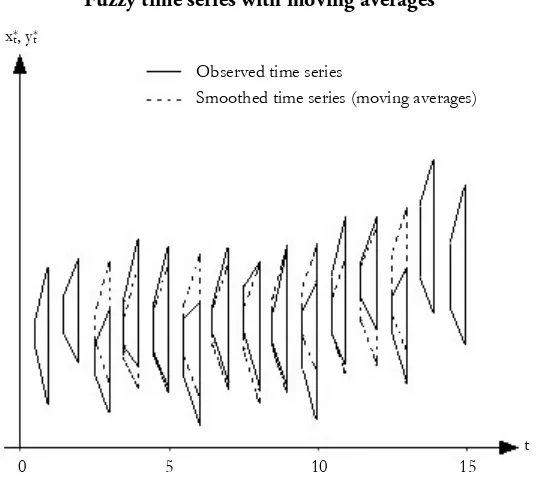
As an example, let T= {1,2,3,…,15} and a fuzzy time series ∗ with trapezoidal characterising functions, that ( ∗) ( ) = ∗( , , , ) _{( )} . As results

the smoothed time series ( ∗₎

( ) are shown (trapezoids with dashed line) in

Figure 4.

Figure 4

Fuzzy time series with moving averages

The filtered time series is smoother if more observations are considered for the filtration, i.e. larger q, with exceptions on the boundaries where the filtered values cannot be obtained. On the other hand, the smoothed time series ( ∗) is shorter than the original time series ( ∗).

Fuzzy predictive densities

In Bayesian inference, probabilities of events A∈ based on a fuzzy probability density f*_{(⋅) are relevant. The standard predictive density for stochastic model X~}

f(⋅|θ); θ∈⊝, based on data D, is defined as marginal density of the stochastic quantity X of (X, ), that is the following:

( | ) ≔_{⊝ ( | ) ( | ) ∀ ∈} ,

where Mx is the observation space of X and (∙ | ) is the a-posteriori density of

the parameter. Fuzzy probability densities are a more general form of expressing a-priori information concerning the parameters θ in stochastic models f(⋅|θ), θ∈⊝. The generalisation of the predictive density for fuzzy a-posteriori densities *_(⋅|D*₎

based on fuzzy data D* _{is possible in the following way (Viertl–Sunanta 2013):}

xt*, yt*

t

0 5 10 15

Observed time series

Let Dδ be the set of all standard probability densities h(·) on ⊝ with δ(θ|D*) ≤

h(θ) ≤ _δ(θ|D*_{) θ∈}⊝_{; δ(θ) and δ(θ) are lower and upper bounds of the}

densities at each δ-level.

In case of fuzzy a-posteriori density *_(⋅|D*_{), the integration has to be generalised}

accordingly. This generalised integration yields fuzzy intervals as a result. Based on

D_δ, the generating family of intervals [a_δ,b_δ], δ∈(0,1] is defined by

aδ≔inf {_⊝ ( | )ℎ( ) : h∈D_δ}

bδ≔sup{_⊝ ( | )ℎ( ) : h∈D_δ}.

Definition 3: The fuzzy predictive density p*(⋅|D*_{) is defined by its values y}* ₌

p*(x|D*_{) ∀} ∈ _{, whose characterising function ψx(⋅) is given, through the}

construction lemma (see also Viertl 2011), by

ψx(y) = sup{δ. [a_{δ ,} b_δ](y): δ∈[0,1]} ∀y∈ℝ, where [a₀ ,b₀] ≔ℝ.

In other words, the fuzzy value of the generalised predictive density is defined via the family of nested compact intervals [a_δ,b_δ]. The fuzzy predictive distribution is used in making probabilistic statements of the unobserved without explicit conditioning on parameters θ, but with conditioning on previously collected fuzzy data D*_.

Fuzzy data in databases

As part of building a complete system, data and information are obtained, analysed, and stored in databases. The important information generally comes from different sources and often cannot be replicated, such as estimation from human experts who describe their knowledge about the areas of interest in natural languages, sensory measurements and mathematical models derived according to physical laws with respect to the systems of interest. Many practical applications require data management components that provide support for managing uncertain data. There are different types of uncertain data: imprecise, vague, ambiguous, inconsistent and incomplete data (Popat–Sharda–Taniar 2004). Fuzzy theory allows us to develop models for imprecise or vague data, in other words, to integrate the vague knowledge into databases. To store this type of information, fuzzy databases are necessary for storing fuzzy data.

realistic information concerning real data. Fuzzy numbers and fuzzy vectors can be represented in databases by storing δ-cuts. In addition, fuzzy multivariate data can be represented in databases by storing a suitable family of δ-cuts of the corresponding vector-characterising function. Learning how to store fuzzy data in traditional relational databases is critical to satisfying the normal forms and keeping the integrity of a database through the fuzzy model of a relational database. A fuzzy meta-model keeps all relevant fuzzy data and manages links to the relations of real entities (see also Hudec 2016 for details).

Final remarks

In regional studies, measurements are crucial in data collection for further statistical analyses. These measurements of continuous variables are uncertain, or more or less fuzzy. The fuzziness of individual measurement results can be described by so-called fuzzy numbers, whereas the variability and errors are described by stochastic models. As a result, the analysis of repeated measurements is possible using respective generalised statistical methods. In this contribution, some generalised statistical methods to handle the so-called fuzzy data are described. Descriptive statistics provide simple summaries of the collected samples and measures (data). They form the basis of virtually every quantitative analysis of the data. Through concepts of fuzzy numbers and characterising functions, fuzzy data are summarised and represented in forms of fuzzy histograms, which provide more information when memberships of the individual data to different classes are not crisp. Some other statistics, such as fuzzy empirical distribution functions and correlation coefficients, are also useful for preliminary data analysis. For better understanding and future projection of the behaviours of the variables under analysis, models for prediction based on fuzzy information, such as fuzzy regression, fuzzy time series and fuzzy predictive density, have been generalised and introduced.

Fuzziness is everywhere in the physical world. In order to describe different regional facets of reality, the methods have to undertake this type of uncertainty. This is possible, and related methods are available through mathematical models. Accordingly, application of such methods results in more realistic models for data analysis and, subsequently, better understanding of the collected data.

REFERENCES

AMT DER TIROLER LANDESREGIERUNG (2016): Stickstoffdioxid: Grenz- und Richtwerte, Abteilung

Raumordnung-Statistik (downloaded: 8 June 2016)

https://www.tirol.gv.at/umwelt/luft/ diagramm-stickstoffdioxid/

BURROUGH, P. A. (2001): GIS and Geostatistics: Essential Partners for Spatial Analysis

ENE, C. M.–HURDUC, N. (2010): A fuzzy Model to Estimate Romanian Underground

Economy Internal Auditing and Risk Management 2 (18): 1–10.

FEDERAL ENVIRONMENT AGENCY (2002): 6th Report on the State of the Environment in Austria

Wien. (downloaded 8th June 2016)

http://www.umweltbundesamt.at/fileadmin/site/umweltkontrolle/2001/ E-02_luft.pdf

GUGLANI,S.–KATTI,C.P.–SAXENA,P.C. (2013): Fuzzy Statistical Database and Its Physical

Organization International Journal of Database Management Systems 5 (4): 27–47. GULEDA,O.E.–IBRAHIM,D.–HALIL,H. (2004): Assessment of Urban Air Quality in Istanbul

using Fuzzy Synthetic Evaluation Atmospheric Environment 38 (23): 3809–3815. HUDEC,M. (2016): Fuzziness in Information Systems Springer, Switzerland.

KLIR,G.–YUAN,B. (1995): Fuzzy Sets and Fuzzy Logic-Theory and Applications Prentice Hall,

Upper Saddle River.

KOVÁŘOVÁ,L.–VIERTL,R.(2015): The Generation of Fuzzy Sets and the Construction of

Characterizing Functions of Fuzzy Data Iranian Journal of Fuzzy Systems 12 (6): 1–16.

LANDESINSTITUT FÜR STATISTIK (ASTAT) (2015): Statistisches Jahrbuch für Südtirol Autonome

Provinz Bozen, Bozen, Südtirol.

LEE,E.S. (1995): Fuzzy Spatial Statistics In: Selected Papers of Engineering Chemistry and Metallurgy

pp. 151–157., Institute of Chemical Metallurgy, Chinese Academy of Science, China.

POPAT, D.–SHARDA, H.–TANIAR, D. (2004) Classification of Fuzzy Data in Database

Management System In: NEGOITA, M. G. (Ed.) Proceedings of Knowledge-Based

Intelligent Information and Engineering Systems pp. 691–697., 8th International

Conference, New Zealand.

SERRANO,J.M.–VILA,M.A.–ARANDA, V.–DELGADO,G. (2001): Using Fuzzy Relational

Databases to Represent Agricultural and Environmental Information Mathware &

Soft Computing 8: 275–289.

SHAPIRO, A. F. (2006): Fuzzy Regression Models In: Proceedings of Actuaries Research

Conference (ARC), Instituto Tecnológico Autónomo de México (ITAM), Mexico, August 11-13, 2005, Society of Actuaries, IL.

SHIANG-TAI,L.–CHIANG,K. (2002): Fuzzy Measures for Correlation Coefficient of Fuzzy

Numbers Fuzzy Sets and Systems 128 (2): 267–275.

TANAKA, H.–UEJIMA,S.–ASAI, K. (1982): Linear Regression Analysis with Fuzzy Model

IEEE Transactions on Systems, Man and Cybernetics 12 (6): 903–907.

VIERTL,R. (2011): Statistical Methods for Fuzzy Data Wiley, Chichester.

VIERTL,R. (2015): Measurement of Continuous Quantities and their Statistical Evaluation

Austrian Journal of Statistics 44 (1): 25–32.

VIERTL, R.–SUNANTA, O. (2013): Fuzzy Bayesian Inference METRON (Fuzzy Statistical

Analysis: methods and applications) 71 (3): 207–216.

WICHERN,D.W.–JOHNSON,R.A. (2007): Applied Multivariate Statistical Analysis 6th _{ed., Pearson}