Munich Personal RePEc Archive
Causal latent Markov model for the
comparison of multiple treatments in
observational longitudinal studies
Bartolucci, Francesco and Pennoni, Fulvia and Vittadini,
Giorgio
University of Perugia, University of Milano-Bicocca, University of
Milano-Bicocca
August 2015
Online at
https://mpra.ub.uni-muenchen.de/66492/
Causal latent Markov model for the comparison of multiple treatments in
observational longitudinal studies
Francesco Bartolucci
Department of Economics
University of Perugia (IT)
email: [email protected]
Fulvia Pennoni
Department of Statistics and Quantitative Methods
University of Milano-Bicocca (IT)
e-mail: [email protected]
Giorgio Vittadini
Department of Statistics and Quantitative Methods
University of Milano-Bicocca (IT)
e-mail: [email protected]
September 7, 2015
Abstract
We extend to the longitudinal setting a latent class approach that has beed recently introduced by Lanza et al. (2013) to estimate the causal effect of a treatment. The proposed approach permits the evaluation of the effect of multiple treatments on subpopulations of individuals from a dynamic perspective, as it relies on a Latent Markov (LM) model that is estimated taking into account propensity score weights based on individual pre-treatment covariates. These weights are involved in the expression of the likelihood function of the LM model and allow us to balance the groups receiving different treatments. This likelihood function is maximized through a modified version of the traditional expectation-maximization algorithm, while standard errors for the parameter estimates are obtained by a non-parametric bootstrap method. We study in detail the asymptotic properties of the causal effect estimator based on the maximization of this likelihood function and we illustrate its finite sample properties through a series of simulations showing that the estimator has the expected behavior. As an illustration, we consider an application aimed at assessing the relative effectiveness of certain degree programs on the basis of three ordinal response variables when the work path of a graduate is considered as the manifestation of his/her human capital level across time.
1
Introduction
We propose a causal inference approach, based on a Latent Markov (LM) model, to dynamically evaluate the
average effect of multiple treatments in a longitudinal context in which multivariate responses are observed
at different time occasions. For this aim, we formulate the LM model (Bartolucci et al., 2013) within a
Potential Outcome (PO) conceptual approach (Rubin, 1974, 2005), and we propose to estimate this model
using a Propensity Score (PS) method (Imbens, 2000). An estimator of causal effects results, which is based
on a weighted likelihood function, with weights computed according to the PS approach; this estimator may
be used in order to evaluate the efficacy of a treatment versus another one on different subpopulations across
time.
In experimental settings, techniques for estimating causal effects with more than two treatments have
been used for many years. This issue is also of great interest in non-experimental settings, where the need
arises of estimating causal effects on the basis of observational data. In this regard, the PO framework is of
particular interest as it allows us to define causal effects in a straightforward way and to formulate techniques
for their estimation. In its original formulation, a set of POs corresponding to the possible treatments is
assumed to exist for every sample unit, but it is possible to observe only the outcome corresponding to the
taken treatment. This “missingness” problem is the primary challenge of causal inference and, therefore,
suitable methods have been proposed in order to overcome it and then obtain reliable estimators of the
causal effects defined in terms of summary statistics of the individual differences between POs. Among
these measures, the Average Treatment Effect (ATE) is of particular relevance. It is defined as the average,
over the population under study, of the difference between the POs corresponding to two treatments of
interest or between the treatment of interest and a control. As other causal effects, ATE may be estimated
by a PS method (see, among others, Rosenbaum and Rubin, 1983; Imbens, 2000; Guo and Fraser, 2010),
so as to balance the groups corresponding to the different treatments, taking into account pre-treatment
covariates. In practice, the estimate of the effect of interest, such as ATE, is computed by using matching
methods, as in (Angrist, 1991), or by weighting estimators similar to those proposed by Robins et al. (2000).
As noted by many authors, PS weighted estimators follow the well-known sampling theory approach of
Horvitz and Thompson (1952) for estimating a population total. Some generalizations have been proposed
by Hirano et al. (2003); see also Hern´an et al. (2001). It also worth noting that McCaffrey et al. (2013)
recently introduced an innovative use of PS weights to control for pre-treatment unbalances on the basis of
observed variables in non-randomized/observational studies. The authors suggested an operative pathway
to implement PS weighting for multiple treatments using generalized boosted models.
tradi-tional sense and methods of causal inference based on the PO approach. Along these lines, Lanza et al.
(2013) proposed a PS based method for making causal inference in connection with the Latent Class (LC)
model (Lazarsfeld and Henry, 1968; Goodman, 1974). This approach considers both matching and weighting
on the basis of individual PSs depending on pre-treatment covariates. In this paper, we extend the proposal
of Lanza et al. (2013) to a longitudinal context in which different measurement occasions are considered
after the treatment. In this regard it is worth considering that, in economic and social contexts, we can
easily dispose of longitudinal observational datasets and often the focus is on the study of the effect of
a policy or treatment on certain outcomes of interest, accounting also for the evolution of such an effect
across time on different subpopulations of interest. In the estimation of causal effects, longitudinal data are
generally preferable to cross-sectional data; see, among others, Aalen et al. (2012) and Arjas (2013) and the
winter 2014 issue ofEconometric Theory, which gives a comprehensive discussion about methods of causal inference.
As already mentioned, the approach we propose is based on the LM model, which is an important
statistical model that may be conceived as an extended version of the LC model having a longitudinal
dimension. The LM model dates back to Wiggins (1955), who introduced it to analyze latent changes on
the basis of panel data. This initial version is based on a homogeneous Markov chain and may be used
with a single outcome at each time occasion. Wiggins (1955) formulated the model so that the manifest
transition is a mixture of the true change and a spurious change due to measurement errors in the observed
states. Among the main extensions of the basic version of the LM model we mention: those based on the
inclusion of constraints on the measurement component or on the latent structure of the model (Bartolucci,
2006); those based on the inclusion of individual covariates (Vermunt et al., 1999; Bartolucci and Farcomeni,
2009); those to deal with multilevel longitudinal data (Bartolucci et al., 2011). For a thorough review see
Bartolucci et al. (2013, 2014) and Pennoni (2014).
One of the novelties of the proposal we formulate in this article relies on the adopted parameterization of
the latent process, so as to express causal effects in terms of transition between latent states corresponding to
subpopulations characterized by different conditions of interest for the study. Moreover, it is also innovative
the use of a PS method for the estimation of the causal LM model, which is formulated following a PO
approach. In practice, we implement a weighted maximum likelihood estimator based on two steps. At
the first step, the probability of choosing a certain treatment on the basis of the pre-treatment covariates is
estimated by means of a multinomial logit model. At the second step, a weighted version of the log-likelihood
of the LM model, with weights depending on the estimates computed at the first step, is maximized. In
we use a non-parametric bootstrap method (Davison and Hinkley, 1997).
Overall, with multiple treatments and multivariate longitudinal data, the proposed approach allows us
to reliably estimate ATEs in terms of initial and transition probabilities between different latent states.
In practice, these latent states summarize the different configurations of the outcomes observed at each
time occasion. In the proposed formulation the response variables are categorical, but it may be simply
generalized to deal with any kind of response variable.
The remainder of this article is organized as follows. The next section outlines the traditional LM
model framework. Section 3 provides a technical illustration of our proposal, focusing in particular on the
assumptions of the causal LM model and the parametrizations adopted to express causal effects. Section
4 illustrates the two-step estimator of the proposed model based on a PS weighting scheme. Section 5
deals with the consistency of the proposed estimator of the treatment effects and illustrates, under different
scenarios, its finite sample properties by means of a simulation study. Section 6 describes an application
focused on the evaluation of the effect of different academic degrees based on data collected in the Lombardy
region (Italy). In the last section we provide some concluding remarks.
2
Standard latent Markov model
Let n denote the number of individuals that are longitudinally observed and let T denote the number of time occasions. With reference to individualiand occasiont,i= 1, . . . , n,t= 1, . . . , T, we observe a vector of r categorical response variables Yit = (Yi1t, . . . , Yirt). Each response variable Yijt, j = 1, . . . , r, has cj categories, labeled from 0 to cj−1. For every individual iand time occasiont we also consider a vector of covariates Xit. Throughout this article we denote a realization of random variables or vectors with the
lower case.
The variable of main interest in the present approach is a latent variable that is individual- and
time-specific; moreover, it has a discrete distribution with support{1, . . . , k}for which more details are provided below. For individual i and time occasion t, this variable is denoted by Hit, given its nature of hidden variable, and for the same individual i we introduce the latent vector Hi = (Hi1, . . . , HiT). We assume that the variables in Yit are conditionally independent given Hit (local independence); we also assume conditional independence between the response variables at different time occasions given the latent process.
Note that the assumption that the latent variables are discrete corresponds to defining a certain numberk
of latent classes (or latent states) of individuals, with individuals in the same class having the same latent
with reference to the response variables.
Among the available parametrizations for LM models, in terms of distribution of the response variables
and the latent variables, that proposed by Bartolucci et al. (2011) is of particular interest. The resulting
model is suitable to deal with educational data having a multilevel structure, due to students collected in
classes. Under this model, which is formulated for binary outcomes, the conditional distribution of the
response variables given the latent variables is parameterized as
p(Yijt= 1|Hit=h) =
exp(ξh−νjt) 1 + exp(ξh−νjt)
, h= 1, . . . , k, j= 1, . . . , r, t= 1, . . . , T, (1)
under the constraint of monotonicityξ1<· · ·< ξk, whereξh is theh-the level of the latent trait character-izing the student, and νjt is the difficulty level of itemj administered at occasion t. The above constraint of monotonicity on the parameters inξ = (ξ1, . . . , ξk)′ is typically adopted in the item response theory (see, among others, Hambleton and Swaminathan, 1985). This constraint may be also formulated for the case of
ordinal response variables, so that the latent classes (or latent states) corresponding to the different values
of Hit are suitably ordered (see also Bartolucci et al., 2013).
Under the model of Bartolucci et al. (2011), the initial and transition probabilities of the latent process
are parameterized using global logits (McCullagh, 1980). Ignoring for simplicity the multilevel structure,
with reference to the initial probabilities we have
logp(Hi1 >h)
p(Hi1 < h)
=αh+x′i1β, h= 2, . . . , k.
Concerning the transition probabilities we have
logp(Hit>h|Hi,t−1 = ¯h)
p(Hit< h|Hi,t−1 = ¯h)
=γ¯hht+x′itδt,
for ¯h = 1, . . . , k, h = 2, . . . , k, and t = 2, . . . , T. The intercepts in the above expressions depend on the level of the latent variable and β and δt are vectors of regression coefficients for the individual covariates.
In this article, we adopt a related parametrization that does not require the constraint of monotonicity so
that the conditional distribution of each response variable, given the corresponding latent variable, is free.
3
Causal latent Markov model
“potential versions” of the latent variables Hit, which are denoted by Hit(z), i = 1, . . . , n, t = 1, . . . , T,
z= 1, . . . , l, wherel is the number of the possible treatments. In particular,Hit(z) corresponds to the latent state of individual i at occasiont if he/she had taken treatment z. The sequence of these variables for the same individual iis collected in the vector H(z)i = (Hi1(z), . . . , HiT(z)) and their distribution may arbitrarily depend on the pre-treatment covariates. As in typical PO approaches, this dependence is not explicitly
modeled; more details about this point are provided at the beginning of Section 5.
VariablesHit(z) are not directly observable for any z. This is because, as in a typical problem of causal inference, only one of the possible outcomes Hit(z) is indeed selected and this selection may depend on the value of the variables themselves. Moreover, in the present context there is a further reason that
complicates the inference: the variable of interest is not directly observable even for the selected treatment.
This is because it is a latent variable that affects the response vector Yit, and then it is only indirectly
observable through this vector.
Regarding the latent processesH(z)i , we assume that they follow a first-order Markov chain. The initial
probabilities are modeled through a multinomial parametrization depending on the treatment and that is
alternative to the parametrization illustrated at the end of the previous section. In particular, regarding
the initial and transition probabilities we assume a baseline-category logit model which does not require any
ordering of the latent states. Regarding the initial probabilities, we assume that
logp(H (z) i1 =h)
p(Hi1(z) = 1) =αh+
d(z)′βh, h= 2, . . . , k, (2)
whereαh is the intercept, βh = (βh2, . . . , βhl)′ is a column vector of l−1 parameters, andd(z) is a column vector of l−1 zeros with the (z−1)-th element equal to 1 ifz >1. In this way, for z >1, the element βhz of βh corresponds to the effect of the z-th treatment with respect to the first treatment. More precisely, this is an ATE as it is referred to the whole population of interest. For instance, β22 being positive means that the second type of treatment increases the probability that the individual is in latent class 2
with respect to first treatment. On the other hand, it is worth noting that, due to the discrete nature of
the treatment indicator z, equation (2) does not impose any restriction on the marginal distribution of
Hi1(z). Moreover, in order to measure ATE for comparing two treatments, we can directly use comparisons of the type p(Hi1(z) =h)−p(Hi1(1) =h) forz = 2, . . . , l, which are expressed on the probability rather than on the logit scale. Finally, in terms of causal effects, a comparison different from that using the first type
of treatment as reference category may be simply based on the difference between suitable elements of βh.
difference βh3−βh2 or p(Hi1(3) =h)−p(H (2)
i1 =h), which are again ATEs. Obviously, in an application all these effects will be based on parameter estimates which are computed as described in Section 4.
The transition probabilities of the hidden chain are modeled as follows:
logp(H (z) it =h|H
(z) i,t−1 = ¯h)
p(Hit(z)= 1|Hi,t(z)−1= ¯h) =γ¯hh+d(z)
′δ
h, ¯h= 1, . . . , k, h= 2, . . . , k, t= 2, . . . , T. (3)
The parameters to be estimated in this case are the intercepts γ¯hh and the vectors of regression coefficients in δh = (δh2, . . . , δhl)′, h = 1, . . . , k. In particular, each coefficient δhz is again an ATE which, however, is referred to the transition from level 1 to level h of the latent variable. This effect has an interpretation similar to the one given above in terms of difference on the logit scale between a certain treatment and the
first treatment. On the other hand, even in this case we can conceive an ATE directly measured on the
probability scale, having expression p(Hit(z) = h|Hi,t(z)−1 = ¯h)−p(Hit(1) = h|Hi,t(1)−1 = ¯h), with ¯h = 1, . . . , k,
h = 2, . . . , k, or p(Hit(z) = h)−p(Hit(1) = h), after having properly elaborated the initial and transition probabilities of the Markov chain. Comparisons between two arbitrary treatments in terms of causal effect
are also possible and may be based on differences between the corresponding elements of the vectorδh, such
as δh3−δh2, or between transition probabilities, such as p(Hit(3) =h|H (3)
i,t−1 = ¯h)−p(H (2)
it =h|H (2)
i,t−1 = ¯h) with ¯h= 1, . . . , k,h= 2, . . . , k.
About the parametrization adopted in the proposed model, we clarify that no constraints are assumed
on the distribution of every response variableYijt given the corresponding latent variable Hit(z). Therefore, this distribution depends on the following parameters:
φjy|h =p(Yijt=y|Hit(z)=h), h= 1, . . . , k, j = 1, . . . , r, y = 0, . . . , cj−1.
The above conditional distribution of the response variables at a specific time occasion, given the
corre-sponding latent state, helps to identify the latent states. Such probabilities may be parametrized as in
equation (1), but in the present context we avoid this or similar parametrizations in order to obtain a more
flexible model.
The above assumptions incorporate in the model the belief that the only variables that have a direct
effect on the outcomes are the latent variables. In particular, local independence means that if the latent
variable for an individual at a given occasion was known, the knowledge of an outcome would not help in
predicting the other outcomes for the same occasion. Obviously, this does not rule out an effect of the
therefore, a fundamental role. It is also worth noting that the latent variables, as in the model presented
in Section 2, are conceived as discrete with k possible values. This allows us to consider a semi-parametric distribution that is parsimonious and based on parameters which are easy to interpret. It is also well known
that this assumption allows the model to properly fit the data, as shown in many applications (see also
Bartolucci et al., 2013), giving more flexibility to the latent structure with respect to using continuous latent
variables. Finally, using discrete latent variables simplifies the computation of the manifest distribution of
the response variables given the covariates as it avoids the use of integrals, which are instead necessary with
continuously distributed latent variables.
Note that assumptions similar to the previous ones may be formulated with continuous outcomes and
also outcomes of a mixed nature can be dealt with. For instance, if some of the outcomes are continuous,
these may be modeled by assuming a suitable conditional parametric distribution, such as the Normal
distribution, with parameters depending on the latent classes, as in a finite mixture model (McLachlan and
Peel, 2000). This makes the proposed approach flexible enough to deal with very different contexts in which
longitudinal data are observed and causal effects have to be estimated with reference to the dynamics of the
response variables induced by the treatment.
Regarding the treatment selection mechanism, we formulate the following assumptions which are typical
of the causal inference literature:
• we assume the consistency rule according to whichHit=Hit(zi), wherezi is the observed treatment of individual i;
• we assume that 0 < p(Zi = z|xi) < 1 for z = 1, . . . , l and any possible configuration xi of the pre-treatment covariates. In this way, every unit has a positive probability of taking each possible
treatment;
• absence of unmeasured confounding according to which Zi |= Hi(z)|Xi,z= 1, . . . , l.
The combination of the last two assumptions is referred to asstrong ignorabilityby Rosenbaum and Rubin (1983). This means that, given the pre-treatment covariates, the choice of the treatment is independent of
the potential outcomes.
4
Two-step maximum likelihood estimation
In order to estimate the causal model formulated in the previous section and following Lanza et al. (2013),
McCaffrey et al., 2013). At the first step, we estimate a model for the probability of taking a certain type
of treatment given the individual pre-treatment covariates. At the second step, we estimate the assumed
LM model by maximizing a weighted version of the log-likelihood for this model, with weights based on the
parameter estimates from the previous step. It must be clear that the observed data consist, fori= 1, . . . , n, of the vector of pre-treatment covariatesxiand the received treatmentzi, further to the time-specific vectors of responsesyi1, . . . ,yiT.
In more detail, the first step of the proposed method consists in estimating a multinomial logit model
based on the assumption
logp(Zi =z|xi)
p(Zi = 1|xi)
=ηz+x′iλz, z= 2, . . . , l, (4)
where ηz and λz are regression parameters. On the basis of the parameter estimates, we compute the individual weights
ˆ
wi=n
1/pˆ(zi|xi) Pn
m=11/pˆ(zm|xi)
, i= 1, . . . , n. (5)
Note that these weights are rescaled so that their sum is equal to the sample size, that is, Pn
i=1wˆi = n; this is necessary for the model selection as we explain below. Moreover, as we illustrate in the application
in Section 6.2, the actual set of pre-treatment covariates must be chosen appropriately; see also McCaffrey
et al. (2013).
At the second step, we maximize the weighted log-likelihood
ℓ(θ) = n X
i=1 ˆ
wiℓi(θ), ℓi(θ) = logp(yi1, . . . ,yiT|zi), (6)
where θ is the vector of all LM model parameters arranged in a suitable way. The manifest probability
p(yi1, . . . ,yiT|zi) is computed by suitable recursions developed in the hidden Markov literature (Baum et al., 1970; Welch, 2003; Zucchini and MacDonald, 2009) on the basis of the probabilities p(yit|Hi(t)=h) and the initial and transition probabilities of the corresponding hidden Markov chain parametrized as in
equations (2) and (3). Given the assumption of local independence described above, we have that
p(Yit=y|Hit=h) = r Y
j=1
φjyj|h,
wherey= (y1, . . . , yr) is a generic configuration ofYit.
The above model log-likelihood may be maximized with respect toθby using the Expectation-Maximization
dis-crete latent variable models; see Bartolucci et al. (2013), Chapter 5, for details about its implementation
for LM models. The EM algorithm is based on the concept of complete data, which correspond to the value of every latent variable, further to the observed covariates and response variables. Therefore, after some
algebra, thecomplete data log-likelihood is given by
ℓ∗(θ) = k X h=1 r X j=1 T X t=1 cj−1
X
y=0
ahjtylogφjy|h+ k X h=1 n X i=1 ˆ
wibhi1logp(Hi1 =h|zi)
+ k X ¯ h=1 k X h=1 n X i=1 T X t=2 ˆ
wib¯hhitlogp(Hit=h|Hit= ¯h, zi), (7)
whereahjtycorresponds to the (weighted) frequency of subjects responding byyto thej-th response variable and belonging to latent state h at occasion t, bhit is an indicator variable equal to 1 if subject i belongs to latent class h at occasion t, with p(Hi1 = h|zi) being the initial probabilities computed according to equation (2), andb¯hhit=bhi,t¯ −1bhit is an indicator variable equal to 1 if the same subject moves from state ¯h to stateh at occasion t, withp(Hit=h|Hit = ¯h, zi) being the transition probabilities computed according to equation (3).
Since the latent configuration is not known for each individual, the EM algorithm maximizes the
log-likelihood above by alternating the following two steps until converge:
• E-step: compute the expected value of the frequencies and indicator variables in (7), given the observed data and the current value of the parameters, so as to obtain the expected value ofℓ∗(θ);
• M-step: update θ by maximizing the expected value of ℓ∗(θ) obtained above.
To select the number of latent states k, when this number is not a priori known, we rely on the Bayesian Information Criterion (BIC; Schwarz, 1978), which relies on an asymptotic approximation of a
suitable transformation of the Bayesian posterior probability of a candidate model. In practice,kis selected on the basis of the observed data through the index
BIC =−2ℓ(ˆθ) + log(n)#par, (8)
where ℓ(ˆθ) denotes the maximum of the weighted log-likelihood and #par denotes the number of free parameters. Note that, due to the definition of the weights given in (5), the sample size is n also after the application of these weights, asPn
i=1wˆi =n, and then the penalization term in (8) is correctly specified. Once parameter estimates have been computed on the basis of the above two-step procedure, we obtain
based on re-sampling subjects (with all their observed pre-treatment covariates, treatment, and outcomes)
a suitable number of times with replacement from the observed sample and computing the estimate of the
parameters for every bootstrap sample. In this way, we suitably take into account the two-step nature of
the proposed estimation method.
5
Properties of the proposed approach
In this section we describe the main asymptotic and finite-sample properties about the proposed approach.
Asymptotic properties, which are dealt with in the following section, are based on standard results about
maximum likelihood estimators, whereas finite-sample properties are studied by simulation.
Before introducing the technical details, it is important recalling that the causal LM model described in
Section 3 may be seen as a marginal model in the sense of Robins et al. (2000). In fact, we do not explicitly
formulate assumptions on the conditional distribution of the latent variables Hit(z) given the pre-treatment covariates Xi, but we model the marginal distribution of these variables. On the other hand, in order to
study the properties of the proposed approach, and in particular implementing the simulation study, we
have to consider a data generating model in which the relation between covariates and latent variables is explicit.
5.1 Asymptotic properties
The data generating model is based on the following scheme for i= 1, . . . , n:
1. the vector of covariates xi is drawn from an unknown distribution f(x);
2. given xi, the potential latent outcomes Hit(z) are drawn, for t = 1, . . . , T and z = 1, . . . , l, from a Markov chain based on initial and transition probabilities which arbitrarily depend on the covariates;
3. givenxi, the treatment indicator zi is generated from a multinomial logit model based on the proba-bilities pz(xi), z= 1, . . . , l, and formulated as in equation (4);
4. the latent variables Hit are generated asHit=Hit(zi) fort= 1, . . . , T;
5. given the generated value of Hit, the outcomesYijt are generated, for j = 1, . . . , r and t = 1, . . . , T, according to the LM model as specified in Section 3.
As already mentioned, the causal LM model that we estimate is a “marginalized” version of the data
proposed estimator, which is illustrated in Section 4, a crucial issue is determining what is the true value
of the parameters of this causal model under the data generating model; the corresponding true parameter
vector is denoted byθ0. A natural way to defineθ0 is as the point of convergence of the standard maximum
likelihood estimator of ˜θ of θ under a “randomized” version of the assumed data generating model; this
estimator is obtained from the maximization of the target function
n X
i=1
ℓi(θ). (9)
The randomized sampling scheme is based on the same steps 1-5 indicated above, but at the third step the treatment indicator variable is drawn from a uniform distribution, which is independent of Xi, with
probabilities pz0 = 1/l, z = 1, . . . , l. Note that the proposed estimator ˆθ and the estimator ˜θ are indeed based on two different sampling schemes, with the first possibly affected by selection bias.
In the following, we establish the consistency of the proposed estimator which is based on the fact that
this estimator and the randomized one are based on the maximization of two functions that, divided by n, converge in probability to the same function as the sample size increases.
Proposition 1. As n → ∞, the estimator θˆ under the data generating model described above and the estimator ˜θ under the randomized sampling scheme converge in probability to the same point θ0 of the
parameter space.
Proof. See Appendix.
A final point we here discuss regards the properties of BIC to select the appropriate number of latent
statesk. In dealing with standard finite mixture models, the consistency of this criterion has been established in Keribin (2000), where consistency means that the true number of mixture components is selected with
probability approaching to 1 as n → ∞. Moreover, McLachlan and Peel (2000) suggests this criterion as suitable in typical applications of mixture models and, similarly, Bacci et al. (2013) showed, on the basis
of a deep simulation study, that it tends to outperform alternative selection criteria for the traditional LM
model. Moreover, advanced versions of BIC have been recently introduced and studied from the point of
view of consistency when the assumed statistical model is estimated by composite, instead of full, composite
likelihood; see Gao and Song (2010).
In the present causal framework, the above results are not directly applicable essentially for two reasons.
First, the estimated model is not directly the data generating model, but a “marginalized” version of this
one. Second, the adopted estimator is not a standard likelihood estimator neither a composite likelihood
illustrated. This conclusion is supported by the simulation results that are illustrated in the following
section.
Regarding the choice of the number of latent states, our point of view is that it is not essential to
spot the “correct” number of latent states only on the basis of the observed data in a causal model as the
present one. In fact, reasons of interpretability and stability of the results may lead to choosing a different
number of latent states with respect to that indicated by a selection criterion. Moreover, adopting solely a
selection criterion based on the observed data may lead to choosing an increasing number of states as the
number of time occasions T increases. In fact, as T increases, the differences between individuals in terms of observable path tend to increase and it is easier to spot these differences as the amount of information
increases. However, the fact that in the same applicative context and for the same group of individuals
two different values of k may be suggested, depending on the length of the period of observation, may be undesirable from the interpretative point of view.
5.2 Simulation study
In order to study the finite-sample properties of the estimator illustrated in the previous section, we
per-formed a simulation study in which the estimates obtained from this method are compared with those
ob-tained from the naive estimation method of the LM model without using PS weighting and those obob-tained
in the case of randomized treatment. Details about the simulation design and its results are illustrated in
the following.
5.2.1 Simulation design
We assume the existence of two covariates affecting both the treatment and the value of the potential
outcomes Hit(z) for all possible treatmentsz; the first of these covariates (xi1) is continuous and is generated from a standard normal distribution, whereas the second (xi2) is binary with two possible values, -0.5 and 0.5, having the same probability. The observed values of these two covariates are collected in the vector
xi. The simulation is based on the following generating model for the POs at the initial time occasion
logp(H (z)
i1 =h|xi)
p(Hi1(z)= 1|xi)
=α∗h+βhz∗ + (xi1+xi2)τh, h= 2, . . . , k, z= 1, . . . , l,
whereas for the next occasions we have
logp(H (z)
it =h|H (z)
i,t−1 = ¯h,xi)
p(Hit(z)= 1|Hi,t(z)−1= ¯h,xi)
with ¯h= 1, . . . , k,h= 2, . . . , k, and z= 1, . . . , l. Note that in the above expressions we add an asterisk to the parameters αh,βhz,γhh¯ , andδhz, as these parameters are different from those of the causal LM model. In fact, as already explained in Section 5.1, this model does not coincide with the data generating model.
In the base-line simulation design, we assume k = 2 latent states and l = 2 treatments, and we fix
α∗2 =−1, β22∗ = 2, τ2 = 1, γ12∗ = −1, andγ22∗ = 1, with δ∗22 = β22∗ /2 and ψ2 =τ2/2, so that the effect of treatment and covariates is smaller on the initial occasion with respect to the following ones. The assignment
mechanism of the treatment is based on the assumption
logp(Zi= 2|xi)
p(Zi= 1|xi)
=xi1+xi2.
Given the same assignment mechanism, with k= 3 latent states, and again l= 2 possible treatments, we fix α∗
2 = −0.5, α∗3 = −1.5, β22∗ = 1.5, β32∗ = 3, γ12∗ = −1, γ13∗ = −2, γ22∗ = 1, γ23∗ = 0, γ32∗ = 1, γ∗33 = 2,
τ2 = 0.5, andτ3 = 1, withδ∗h2 =βh2∗ /2 andψh =τh/2 for h= 2,3.
Under the scenario with l = 3 treatments, we assume that the treatment is assigned according to the multinomial logit model based on the following assumption:
logp(Zi =z|xi)
p(Zi = 1|xi)
= (z−1)(xi1+xi2), z= 2,3.
Moreover, with k= 2 we use the same values as above for all the parameters of the model for the potential outcomes, with β22∗ = 1 and β∗23 = 2. Similarly, with k = 3 we assume β22∗ = 0.75, β∗23 = 1.5, β32∗ = 1.5, and β33∗ = 3. In both cases we have δhz∗ =βhz∗ for allh and z.
Under each model defined as above, we drew 1,000 samples of sizen= 1000,2000 for a number of time occasionsT = 4,8, so that there are 16 scenarios overall. For every sample, the causal effects were estimated by the proposed method and its unweighted version. Moreover, for comparison, the corresponding estimates
based on a randomized design were obtained. The latter amounts to draw the assignment variablesZi from a generalized Bernoulli distribution with l categories having the same probability, and then independently from the pre-treatment covariates, and applying the unweighted estimator on the resulting data.
5.2.2 Simulation results
approach when samples are affected by confounding is denoted as “proposed”, and the estimator which
does not correct for confounding is denoted as “naive”, being based on the maximization of the standard
(unweighted) likelihood function.
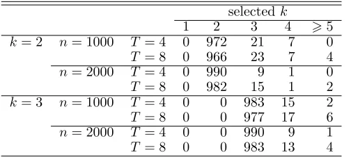
[Table 1 about here.]
[Table 2 about here.]
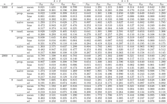
[Table 3 about here.]
[Table 4 about here.]
From the results in Tables 1 and 3, which are obtained under different scenarios, we conclude that
the bias of the proposed estimator is typically negligible. We stress that this bias is computed as the
difference between the mean of the estimates based on the proposed method and that of the estimates
based on the randomized experiment, as we do not directly estimate the parameters of the data generating
model. Therefore, it would not be correct to directly compare, for instance, the average of the estimates
of the parameters βhz with the proposed method with the true value of the parametersβhz∗ assumed in the data generating model. We also find that, as expected, the standard deviation of the proposed estimator
decreases asn andT increase; in particular, it decreases with a rate close to √n.
On the other hand, the bias is typically large for the naive estimator. This bias does not reduce as the
sample size and/or the number of time occasions increases and confirms that, differently from the proposed
estimator, the naive estimator is inadequate and may lead to completely wrong results. These results would
also be very different from those obtainable if the treatment was perfectly randomized.
Finally, it is worth noting that, according to the results in Tables 2 and 4, BIC performs very well
in choosing the optimal number of latent states. Therefore, we conclude that it is an adequate selection
criterion also when the weighted log-likelihood estimator is applied and this justifies the rule in equation (5)
to compute the PS weights.
6
Application
In this section, the proposed methodology is illustrated through an application focused on the estimation
of ATE of the degree type on the Human Capital (HC) development. In particular, we compare individuals
who graduated in different subjects taking into account the university labour market transition in the first
In the following, we first describe the context of the study and the available data. Then, we show
the main results of the application and we provide some remarks about the estimated effectiveness of the
different types of degree.
6.1 Data description
We represent HC by a sequence of individual latent variables having a longitudinal dimension, so as to
study its evolution across time. This follows Heckman (2000), who conceived HC as a latent variable which
is affected by investment in education, individual ability, type of higher education. In turns, HC affects
income, other outcomes (manifest variables) describing the stability of the job position, and skills actually
employed in comparison with the acquired ones.
In order to properly assess the effect of university studies on the transition to the labor market, we
consider the following aspects: (i) different outcomes may describe how much knowledge improves the personal opportunities on the job market, taking into account not only earnings but also indicators of job
stability and improvement in skills; in this regard, Harpan and Draghici (2014) suggested that HC must be
measured also including non-monetary aspects as well as considering its development; (ii) the phenomenon has a longitudinal perspective and the evolution of the outcomes observed at repeated occasions is of main
importance; (iii) the treatment of subjects is not controlled and there are multiple potential treatments corresponding to different types of degree program. Also note that, as in other model frameworks for causal
inference, the pre-treatment covariates are of main importance as the treatment groups differ, already prior
to treatment, in a way that can affect the outcomes. This clearly happens in our application so that the
groups of individuals with different degrees need to be balanced on the basis of these covariates.
The available data derive from certain administrative archives and concern graduates from the Lombardy
region. The Supplementary Material file of the present article provides more details on the administrative
archives from which the data are obtained. The dataset refers to 1,144 individuals who graduated in
2007 from four universities and are resident in the area surrounding Milan. Note that, in this area, these
universities are comparable in terms of prestigious and quality and then we rule out a differential effect
between them in terms of work path. On the other hand, we study the effect of different types of academic
graduation; in other words, the type of graduation is the treatment of interest. For this aim, we deal with a
cohort of graduates who have been observed along four quarters after graduation, covering in this way one
year.
The percentage of the graduates for each type of degree, as well as the descriptive statistics for the
file. In this regard, note thatZi is discrete variable withl= 5 treatments equal to: 1 for technical degrees, 2 for architecture, 3 for economic degrees, 4 for humanities degrees, and 5 for scientific degrees. The groups
are not balanced in terms of pre-treatment covariates; in particular, there are relevant differences between
graduates with a technical degree and those with other degrees.
The followingr = 3 response variables concerning graduates’ employment status are available for each of the four quarters of observation:
i) contract type with categories: none, temporary, and permanent;
ii) skill with categories: none, low/medium, and high;
iii) gross income in Euros (e) with categories: none, 63750 e, and >3750e.
Then, we have r = 3 andcj = 3 for j = 1, . . . , r, as all variables have three response categories. Note that the category none means that the contract type is not temporary neither permanent but some less qualified
type of contract. The category none for skill corresponds to those jobs not requiring any qualified skill, and
for income this category refers to incomes gained from other sources.
Regarding the response variables, note that we essentially distinguish between temporary and permanent
contracts. Moreover, the gross income is reported quarterly and we choose to consider the threshold of
e15,000 yearly, which corresponds to e3,750 quarterly. The third response variable is based both on
skill level and skill specialization. According to the definition of HC given above, the observed response
variables we dispose represent a manifestation of this latent construct. The local independence assumption
is reasonable and, from our point of view, no other dependences in the data need to be specified.
6.2 Results
We first consider the selection of the pre-treatment covariates to be used to compute the weights (first step).
Then, we show the estimated parameters related to ATE of the degree on the work path (second step).
6.2.1 Selection of the pre-treatment covariates
As illustrated in Section 4, the individual weights are computed on the basis of the estimated multinomial
logit model for the treatment, which is based on equation (4).
In general, it is important to select the appropriate pre-treatment covariates that enter in this model;
see also McCaffrey et al. (2013). In this respect, we start from an analysis of the dependence of each of
the analysis is based on an ANOVA model and only covariates for which a clear dependence with the type
of degree is ascertained are included in the multinomial logit model. covariate is considered to have a
strong dependence with the choice of the degree type when the hypothesis is rejected that the means of this
covariate for the different degrees are equal. In the case of qualitative covariates, such as gender, we instead
use a chi-square test of independence for contingency tables. Therefore, we choose the following among the
pre-treatment covariates: gender, district of birth, final grade at high school diploma, type of high school. The parameter estimates of this multinomial model are reported in Table 5.
[Table 5 about here.]
In Table 6 we report some descriptive statistics for the distribution of each of these covariates given the
degree type and accounting for the PS weights based on the fitted multinomial model.
[Table 6 about here.]
From Table 6 we observe that the balance between the groups corresponding to the different university
degrees is considerably higher with respect to the initial distributions (compare with Table 2 in the
Sup-plementary Material file). For instance, the percentage of females among graduates in a technical subject
is around 20% and it is around 80% among graduates in a humanities subject. After re-weighting, these
percentages become equal to 45% and 49%, respectively, and they are close to those computed for the other
university degrees. A similar convergence between the distributions corresponding to the other degree types
is observed for the remaining three covariates.
6.2.2 Results of the model fitting
After the individual PS weights have been obtained, we estimated the proposed LM model for an increasing
number of latent states not larger than 4, so as to avoid models of difficult interpretation, and under this
constraint we selected this number on the basis of BIC, as illustrated in Section 4. It turns out that the
number of latent classes is k = 4 corresponding to the minimum of the BIC index among the values of
k we considered. The corresponding maximum weighted log-likelihood is ℓ(ˆθ) = −5180.00, with 63 free parameters, so thatBIC = 10803.66.
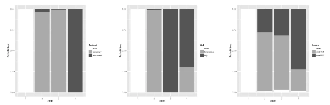
The estimates of the conditional response probabilities (φjy|h) obtained under the selected model with four latent states are reported in Table 7 and are also illustrated in Figure 1.
[Figure 1 about here.]
According to the estimates of the parameters φjy|h we can rather easily interpret the latent states according the corresponding distribution of the response variables. In particular, the first class corresponds
to the cluster of unemployed individuals, and then the probability of the first category is equal to 1 for each
response variable. On the other hand, the fourth latent class corresponds the subpopulation of individuals
in very good work conditions, as they have a permanent contract and tend to have a job with high skill
level and high income. The interpretation of the other two classes is less straightforward, even if it is clear
that they are intermediate between the first class and the fourth. In particular, the second class is that of
individuals that typically have a temporary contract for a low/medium skill job. Individuals in the third
class differ from those in the second for having a higher probability of making use of their high skills. Overall,
the interpretation of these classes in terms of HC may be summarized as follows:
• 1st class: lowest HC level;
• 2nd class: intermediate HC level with high probability of a temporary job, requiring a low/medium skill level, and intermediate income level;
• 3rd class: similar to the 2nd class with the exception of a higher skill level and a slightly higher income;
• 4th class: high HC level with permanent contract, intermediate-high skills, and high income.
It is also worth noting that, although these latent classes can be easily interpreted, they are non-monotonically
ordered, implying that the constraint of monotonicity only holds for certain pairs of classes, such as the pair
(1,4); however, this constraint does not hold for the pair (3,4). Then, avoiding to incorporate in the model
the constraint of monotonicity by parametrizing the conditional response probabilities is a proper choice as
this constraint would reduce the model fit considerably.
The estimates of the regression coefficients αh and βhz affecting the initial probabilities of the hidden Markov chain, see equation (2), are reported in Table 8, with the indication of the significance level for the
test that each of these parameters is equal to 0. For the corresponding estimated initial probabilities see
Table 9. We recall that every parameter βhz may be interpreted as an ATE of degree (treatment) z, with respect to a technical degree (z= 1), in terms of initial probabilities expressed on the logit scale. In Table 8 we also report the estimates of the pairwise differences βhz1 −βhz2, z2 6= z1, which can be interpreted
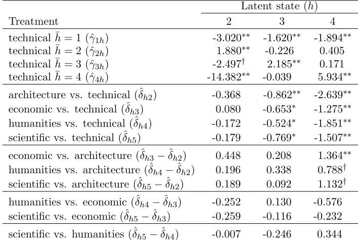
in terms of ATE of treatment z2 with respect to treatment z1. The estimates of the parameters γ¯hh and
significance level for each of these parameters, which may be again interpreted in terms of ATE on the
transition probabilities.
[Table 8 about here.]
[Table 9 about here.]
[Table 10 about here.]
On the basis of the estimates of the logit regression parameters for the initial probabilities, reported in
in Table 8, we conclude that, at the beginning of the period of observation, there is a statistical significant
difference in terms of effect on HC of technical degrees with respect to architecture and humanities degrees
and in favor of the first ones. There is also a significant differential effect of economic degrees with respect
to architecture and humanities degrees. This conclusion is confirmed by the estimated initial probabilities
for each type of treatment given in Table 9, which show that technical and economic degrees have the lowest
probability that a graduate is in the first latent class (0.45 for both degrees) and the highest probability
that he/she in the last latent class ( 0.17 for technical and 0.15 for economic degree). Then, scientific
degrees correspond to intermediate estimates of both probabilities (0.65 for the first class and 0.10 for the
last) whereas, with reference to architecture and humanities degrees, we have the highest probabilities for
the first class (0.75 and 0.67, respectively) and the lowest probabilities for the last class (0.07 and 0.05,
respectively). It is interesting to note that, looking at the initial probabilities of the first or the last class,
we obtain substantially the same ranking of the degree types in terms of effect of initial HC level, an aspect
that gives consistency to our findings. In summary, we can rank the degrees as follows in terms of their
effectiveness at the beginning of the period after graduation: technical, economic, scientific, humanities,
architecture. We rank architecture as the last degree type on the basis of the initial probability of the first
latent class although humanities has a lower probability for the last latent class, but the difference is small.
The picture is somehow different in terms of causal effects of the degree type on the evolution of the HC
level, which is represented through transition probabilities. In fact, on the basis of the estimates of the logit
regression parameters affecting the transition probabilities (Tables 10) we conclude that there are significant
differences between technical degrees and all the other types of degree during the period of observation and
between economic and architecture degrees in favor of the first.
The above conclusions in terms of ranking of the degree types are confirmed by the estimated transition
probability matrices reported in Table 11 for each type of degree and which are computed on the basis of
[Table 11 about here.]
All matrices are characterized by a rather high persistence, with elements in the main diagonal always
greater than 0.65, many of which are also greater than 0.8. However, some differences emerge between these
transition matrices. In order to ease the comparison, it is again convenient to focus on the first and the last
latent classes, corresponding to the subpopulations of individuals with the lowest and the highest HC level,
respectively. In particular, we observe that for technical degrees there is the lowest probability of remaining
in the first latent class (0.72) and then the highest probability of moving away from this class, meaning
that this type of degree induces the best improvement in terms of HC. For this type of degree we also have
the highest probability of remaining in the last class (1.00). The second lowest probability of remaining in
the first class is for economic degrees (0.84), corresponding to the second highest probability of remaining
the last class (0.99). The third lowest probability of remaining in the first class is for humanities degrees
(0.85), corresponding to the second lowest probability of remaining in the last class (0.97). Finally, for
scientific degrees we have the second lowest probability of persistence in the first latent class (0.86) and the
third lowest probability of remaining in the last class (0.97), whereas for architecture we have the highest
probability for the first class (0.89) and the lowest for the last class (0.95).
Overall, we conclude that there is a rather clear ranking between university degrees in terms of impact
on the HC level which is as follows:
• Technical degrees: highest effect at the beginning and in terms of evolution of HC level;
• Economic degrees: impact close to technical degrees and in terms of evolution of HC level;
• Scientific degrees: significantly worse impact with respect to technical and economic degrees;
• Humanities and Architecture degrees: worse effect at the beginning and in terms of evolution of HC level.
In order to assess how these conclusions are sensitive to the initially selected set of covariates, we
performed the same analysis using all the available pre-treatment covariates to compute the individual
weights. This amounts to fit the multinomial logit model, based on equation (4), with all these covariates
and obtain in this way the PS weights. The results of this second fitting are very close to those obtained
above, leading to the same conclusions about the effect of the treatment of interest. For details about this
7
Conclusions
We propose a novel approach for estimating Average Causal Effects (ATEs) when dealing with longitudinal
data in observational studies and in the presence of multiple treatments. It is based on integrating the
Latent Markov (LM) model with modeling techniques based on the potential outcome framework (Rubin,
1974, 2005). We introduce a causal inference perspective into the LM model and, at the same time, we
extend the causal inference approach developed by Lanza et al. (2013) to the longitudinal context. This
innovative statistical method has a potential use in a wide range of observational studies which rely on the
same assumptions. It allows us to summarize the multivariate responses observed at each occasion by latent
classes (or states) having the interpretation of clusters (or subpopulations) of individuals. The flexibility
of the adopted parameterization allows us to deal with any kind of response variable, not only categorical.
Of main importance is the estimation of the ATEs which are expressed in terms of initial probabilities of
the latent classes and transition probabilities between these classes, so as to separate the impact at the
beginning of the period of observation from that on the evolution of the characteristic of interest.
The model is fitted by a two-step maximum likelihood estimation procedure based on first estimating
a multinomial logit model for the probability of taking each type of treatment given suitably chosen
pre-treatment covariates. Then, a weighted log-likelihood of the LM model, with weights computed on the basis
of the estimates computed at the first step, is maximized so as to obtain the parameter estimates. This second
step is based on the expectation-maximization algorithm (Dempster et al., 1977). Reliable standard errors
for the model parameters are obtained by using a non-parametric bootstrap method (Davison and Hinkley,
1997). The number of latent classes is selected by the Bayesian Information Criterion (BIC; Schwarz, 1978).
The selection of the appropriate pre-treatment covariates is made by considering an ANOVA model for
the quantitative covariates and a chi-square test of independence for qualitative covariates. These covariates
are selected if they show a significant dependence with a specific type of treatment. Moreover, the use of the
multinomial logit parameterization for the initial and for the transition probabilities of the latent variables
implies that the number of parameters to be estimated may be potentially high. However, we introduce
a constrained form that makes the model more parsimonious and, in the causal context, this is a suitable
parameterization because it allows us to estimate the effects of interest in case of multiple treatments. A
partially ordered hidden Markov model, as that proposed by Ip et al. (2013), may be also considered.
We assess the asymptotic properties of the proposed estimator by taking into account the data generating
model. We provide a proposition of its consistency by showing that it converges to the same point of the
parameter space at which the standard estimator converges under a perfectly randomized sampling scheme.
study. In this study, we compare the results especially in terms of bias of the proposed weighted estimator
with the naive unweighted estimator of the LM model and with the estimator based on a randomized
assignment of the treatment. As expected, the proposed estimator has a negligible bias, whereas the naive
estimator may have a huge bias. We also evaluate the performance of the BIC and we conclude that this
criterion is able to select the correct number of latent states also when used within the weighted likelihood
approach. According to the simulation study we conclude that the proposed approach leads us to an
adequate estimator of the causal effects of interest.
In the application, we aim at studying the development of the Human Capital (HC), and the related
university-to-work transition phenomenon, due to the different types of degree. We refer to a definition
of HC as a latent construct related to the skills, competencies, and attributes embodied in individuals
that are relevant to the economic activities, with particular reference of the labor market. The response
variables are categorical and they have been chosen in order to capture different aspects of the individuals.
In fact, we conceive HC as a “potential version” of a latent variable which underlies the three employment
quality measures, in accordance with the most recent definitions of HC. Therefore, the local independence
assumption is reasonable. The analyzed data are referred to the first year after graduation of the entire
population of graduates in 2007 in four universities in Milan and certain important pre-treatment covariates
are available. We observe the relevant factors contributing to the treatment assignment and then the
assumption of absence of unmeasured confounders is no doubtful. However, the latter may be also assessed
by a sensitivity analysis which may be considered in subsequent studies. By applying the proposed approach
to the data at hand, we selected a model with four latent states. We show that the results have an easy
interpretation and a rather insensitive to the specification of the multinomial logit model used to obtain
the initial Propensity Score (PS) weights. We conclude that the different types of academic degree have
significantly different effects on the work path. The choice of different treatments (type of degree) has an
impact on the return of investment in HC, the increase of which is higher for those having a technical and
economic degrees respect to other degrees. The model also allows us to rank university degrees in terms of
impact on HC levels. It also worth mentioning that, by applying the same proposal and relaying on more
time occasions, we might study the long term effects of the degrees.
Finally, we stress that the proposed model is very flexible as it may be easily extended to the case of
mixed response variables. Another possible extension of interest is for multilevel data; this extension could
be formulated according to the approach adopted in Bartolucci et al. (2011) where additional discrete latent
variables are introduced to account for the dependence between the individuals in the same clusters. In
PS weights and the second consisting in the maximization of the weighted model likelihood. The main
complication is in this second step and, in particular, in the estimation algorithm. This difficulty is given by
the presence of a complex latent structure based on several latent variables that are dependent each other.
Moreover, special care must be paid to the method for obtaining the standard errors for the parameter
estimates, so as to account for the within-cluster dependence in addition to the two-step nature of the
estimator. As suggested by a Referee, one possibility would be to implement a bootstrap algorithm based
on resampling units within each cluster.
Acknowledgments
We thank the Editor and the Reviewers for many stimulating comments. We are also grateful to Prof. M.
Mezzanzanica and to Dr. M. Fontana, of the Interuniversity Research Centre on Public Services (CRISP),
University of Milano-Bicocca, for providing the analyzed dataset. Finally, we acknowledge the financial
support from the grant RBFR12SHVV of the Italian Government (FIRB project “Mixture and latent variable
models for causal inference and analysis of socio-economic data”). F. Pennoni also thanks the financial
support of the STAR project “Statistical models for human perception and evaluation” funded by the
University of Naples Federico II.
Appendix
Proof of Proposition 1. First of all, consider the average log-likelihood defined according to (6), that is,
¯
ℓ(θ) = ℓ(θ)
n =
Pn
i=11/pˆ(zi|xi) logp(yi1, . . . ,yiT|zi) Pn
i=11/pˆ(zi|xi)
.
Since the parameters of the logit model are consistently estimated at the first step, then also each ˆp(zi|xi) is uniformly consistently estimated and this implies that
¯
ℓ(θ)→p E[1/p(Zi|Xi) logp(Yi1, . . . ,YiT|Zi)] E[1/p(Zi|Xi)]
, (10)
The denominator of (10) may be rewritten as
E[1/p(Zi|Xi)] = l X
z=1 Z
x
[1/p(Zi =z|Xi =x)]p(Zi=z|Xi =x)f0(x)dx
=l,
wheref0(x) refers to the true distribution of the covariates. Using similar arguments, we also have that
E[1/p(Zi|Xi) logp(Yi1, . . . ,YiT|Zi)]
= l X z=1 Z y1 · · · Z yT
f0(y1, . . . ,yT|z) logp(Yi1=y1, . . . ,YiT =yT|Zi =z)dyT· · ·dy1,
where
f0(y1, . . . ,yT|z) = Z
x
p(Yi1 =y1, . . . ,YiT =yT|Xi =x, Zi=z)f0(x)dx
is the conditional distribution ofYi1, . . . ,YiT givenZi, provided thatZiis independent ofXi. Consequently, we have
¯
ℓ(θ)→p E0[logp(Yi1, . . . ,YiT|Zi)], ∀θ,
where the expected value E0(·) is computed under the randomized sampling scheme in which each treatment has the same probability 1/l, so that
E0[logp(Yi1, . . . ,YiT|Zi)]
= 1 l l X z=1 Z y1 · · · Z yT
f0(y1, . . . ,yT|z) logp(Yi1 =y1, . . . ,YiT =yT|Zi=z)dyT · · ·dy1. (11)
Now consider the average version of the target function defined in equation (9), that is,
˜
ℓ(θ) = 1
n
n X
i=1
logp(yi1, . . . ,yiT|zi).
By standard arguments we have that
˜
ℓ(θ)→p E0[logp(Yi1, . . . ,YiT|Zi)], ∀θ.
Therefore, the two target functions on which the two estimators are based convergence to the same function
defined in equation (11). Since usual regularity conditions about the two involved likelihoods are satisfied,
References
Aalen, O. O., Roysland, K., Gran, J. M., and Ledergerber, B. (2012). Causality, mediation and time: a dynamic
viewpoint. Journal of the Royal Statistical Society: Series A, 175:831–861.
Angrist, J. D. (1991). Grouped-data estimation and testing in simple labor-supply models. Journal of Econometrics,
47:243–266.
Arjas, E. (2013). Time to consider time, and time to predict? Statistics in Biosciences, 6:1–15.
Bacci, S., Pandolfi, S., and Pennoni, F. (2013). A comparison of some criteria for states selection in the latent Markov
model for longitudinal data. Advances in Data Analysis and Classification, 8:125–145.
Bartolucci, F. (2006). Likelihood inference for a class of latent Markov models under linear hypotheses on the transition
probabilities. Journal of the Royal Statistical Society, series B, 68:155–178.
Bartolucci, F. and Farcomeni, A. (2009). A multivariate extension of the dynamic logit model for longitudinal data
based on a latent Markov heterogeneity structure. Journal of the American Statistical Association, 104:816–831.
Bartolucci, F., Farcomeni, A., and Pennoni, F. (2013). Latent Markov Models for Longitudinal Data. Chapman &
Hall/CRC, Boca Raton, FL.
Bartolucci, F., Farcomeni, A., and Pennoni, F. (2014). Latent Markov models: a review of a general framework for
the analysis of longitudinal data with covariates (with discussion). Test, 23:433–486.
Bartolucci, F. and Pennoni, F. (2011). Impact evaluation of job training programs by a latent variable model. InNew
Perspectives in Statistical Modeling and Data Analysis, pages 65–73. Springer-Verlag, Berlin.
Bartolucci, F., Pennoni, F., and Vittadini, G. (2011). Assessment of school performance through a multilevel latent
Markov Rasch model. Journal of Educational and Behavioural Statistics, 36:491–522.
Baum, L., Petrie, T., Soules, G., and Weiss, N. (1970). A maximization technique occurring in the statistical analysis of probabilistic functions of Markov chains. Annals of Mathematical Statistics, 41:164–171.
Davison, A. C. and Hinkley, D. V. (1997). Bootstrap Methods and their Application. Cambridge University Press,
Cambridge, MA.
Dempster, A. P., Laird, N. M., and Rubin, D. B. (1977). Maximum likelihood from incomplete data via the EM
algorithm. Journal of the Royal Statistical Society, Series B, 39:1–38.
Gao, X. and Song, P. X.-K. (2010). Composite likelihood Bayesian information criteria for model selection in
high-dimensional data. Journal of the American Statistical Association, 105:1531–1540.
Goodman, L. A. (1974). Exploratory latent structure analysis using both identifiable and unidentifiable models.
Guo, S. and Fraser, M. W. (2010). Propensity Score Analysis: Statistical Methods and Applications. Sage, Thousand
Oaks, CA.
Hambleton, R. K. and Swaminathan, H. (1985). Item Response Theory: Principles and Applications. Kluwer Nijhoff,
Boston.
Harpan, I. and Draghici, A. (2014). Debate on the multilevel model of the human capital measurement. Procedia
-Social and Behavioral Sciences, 124:170 – 177.
Heckman, J. J. (2000). Policies to foster human capital. Research in Economics, 54:3–56.
Hern´an, M. A., Brumback, B., and Robins, J. M. (2001). Marginal structural models to estimate the joint causal
effect of nonrandomized treatments. Journal of the American Statistical Association, 96:440–448.
Hirano, K., Imbens, G. W., and Ridder, G. (2003). Efficient estimation of average treatment effects using the estimated
propensity score. Econometrica, 71:1161–1189.
Horvitz, D. G. and Thompson, D. J. (1952). A generalization of sampling without replacement from a finite universe.
Journal of the American Statistical Association, 47:663–685.
Imbens, G. W. (2000). The role of the propensity score in estimating dose-response functions.Biometrika, 87:706–710.
Ip, E., Zhang, Q., Rejeski, J., Harris, T., and Kritchevsky, S. (2013). Partially ordered mixed hidden Markov model
for the disablement process of older adults. Journal of the American Statistical Association, 108:370–384.
Keribin, C. (2000). Consistent estimation of the order of mixture models. Sankhya: The Indian Journal of Statistics,
Series A, 62:49–66.
Lanza, S. T., Coffman, D. L., and Xu, S. (2013). Causal inference in latent class analysis. Structural Equation
Modeling: A Multidisciplinary Journal, 20:361–383.
Lazarsfeld, P. F. and Henry, N. W. (1968). Latent Structure Analysis. Houghton Mifflin, Boston.
McCaffrey, D. F., Griffin, B. A., Almirall, D., Slaughter, M. E., Ramchand, R., and Burgette, L. F. (2013). A tutorial
on propensity score estimation for multiple treatments using generalized boosted models. Statistics in Medicine,
32:3388–3414.
McCullagh, P. (1980). Regression models for ordinal data (with discussion). Journal of the Royal Statistical Society,
Series B, 42:109–142.
McLachlan, G. and Peel, D. (2000). Finite Mixture Models. Wiley, New York.
Robins, J., Hern´an, M., and Brumback, B. (2000). Marginal structural models and causal inference in epidemiology.
Epidemiology, 11:550–560.
Rosenbaum, P. R. and Rubin, D. B. (1983). The central role of the propensity score in observational studies for causal
effects. Biometrika, 70:41–55.
Rubin, D. B. (1974). Estimating causal effects of treatments in randomized and nonrandomized studies. Journal of
Educational Psychology, 66:688–701.
Rubin, D. B. (2005). Causal inference using potential outcomes: design, modeling, decisions. Journal of the American
Statistical Association, 100:322–331.
Schwarz, G. (1978). Estimating the dimension of a model. The Annals of Statistics, 6:461–464.
Vermunt, J. K., Langeheine, R., and B¨ockenholt, U. (1999). Discrete-time discrete-state latent Markov models with
time-constant and time-varying covariates. Journal of Educational and Behavioral Statistics, 24:179–207.
Welch, L. R. (2003). Hidden Markov models and the Baum-Welch algorithm. IEEE Information Theory Society
Newsletter, 53:1–13.
Wiggins, L. (1955). Mathematical models for the analysis of multi-wave panels. InPh.D. Dissertation, Ann Arbor. Columbia University.
Zucchini, W. and MacDonald, I. L. (2009). Hidden Markov Models for Time Series: An Introduction Using R.
0.00
0.25 0.50 0.75
1.00
1 2 3 4
State Pro b a b il it ie s Contract none temporary permanent 0.00 0.25 0.50 0.75 1.00
1 2 3 4
State Pro b a b il it ie s Skill none lowmedium high 0.00 0.25 0.50 0.75 1.00
1 2 3 4
[image:30.612.52.598.64.239.2]State Pro b a b il it ie s Income none min3750 max3750
Figure 1: Estimated conditional probabilities of labor condition (φjy|h), under the proposed causal LM model