Munich Personal RePEc Archive
Trust and Performance: Exploring
Socio-Economic Mechanisms in the
“Deep” Network Structure with
Agent-Based Modeling
Gao, Lin
21 November 2016
1
Trust and Performance: Exploring Socio-E
conomic Mechanisms in the “Deep”
Network Structure with Agent-Based Modeling
Gao, Lin
Draft: 21 Nov. 2016
Abstract: This paper extends the concept of interaction platforms and explores the evolution of interaction and cooperation supported by individuals‟ changing trust and trustworthiness on directed weighted regular ring network from the angle of micro scope by using agent-based modeling. This agent-based model integrates several considerations below via a relatively delicate experimental design: 1) a characteristic of trust is that trust is destroyed easily and built harder (Slovic, 1993); 2) trustworthiness may be reflected on both strategy decision and payoff structure decision; 3) individuals can decide whether or not to be involved in an interaction; 4) interaction density exists, not only between neighbors and strangers (Macy and Skvoretz, 1998), but also within neighbors; 5) information diffusion. In this agent-based model, marginal rate of exploitation of original payoff matrix and relative exploitation degree between two payoff matrices are stressed in their influence of trust-destroying; influence of observing is introduced via imagined strategy; relationship is maintained through relationship maintenance strength, and so on. This paper treats number of immediate neighbors, degree of embeddedness in social network, mutation probability of payoff matrix, mutated payoff matrix, proportion of high trust agents and probabilities of information diffusion within neighborhood and among non-neighbors as important aspects happening on interaction platforms, and the influences of these factors are probed respectively on the base of a base-line simulation.
Keywords: Trust, trustworthiness, directed weighted regular ring network, agent-based modeling, marginal rate of exploitation, relative exploitation degree, imagined strategy, relationship maintenance strength, number of neighbors, degree of embeddedness in social network, mutation of payoff matrix, information diffusion, social mobility, institutional quality, evolution of interaction, evolution of cooperation
Introduction
Trust as a lubricant permeates almost every aspect of social and economic life. It typically functions on human individuals and is reflected in their social and economic interactions. From the individuals‟ perspective, different personal experiences (including direct interaction experiences and observation experiences) may drive different trust of individuals. At the same time, individuals‟ diverse traits may lead to that their trust gets influenced to different degrees by even the same trust-influencing events. Put another way, individuals would not react to the same degree to external information; there exist people more easily being influenced. Thus, trust is heterogeneous across individuals in a given population, and is more or less subjective.
The micro interactions (interactions of individuals) can be and are often modeled by games, such
Institute of Institutional and Innovation Economics (iino), University of Bremen, Hochschulring 4, WiWi, Room
2
as Prisoners‟ Dilemmas or coordination games et cetera. Cooperation in dilemma-like payoff structure is a remarkable research topic in game theory. (e.g., Axelrod, 1984/2006) In research of trust by modeling micro interactions by non-cooperative Prisoners‟ Dilemmas, diachronic share of cooperation in the whole society (number of cooperation over population size) is often adopted as a measure of (social) trust. This method actually treats global share of trustworthy behaviors as equal to (social) trust and has reasonability, to some extent. However, some possible disadvantages accompany, at the same time. For example, given the payoff structure, this method cannot distinguish the different degrees of influences on an agent of trust-increasing and trust-decreasing events. It implies trust-decreasing events have an equivalent impact with trust-increasing events (even with very opposite directions). But generally speaking, trust is produced harder but can be destroyed easily. Slovic (1993) also states, “It (Trust) typically created rather slowly, but it can be destroyed in an instant by a single mishap or mistake”; the “fragile” nature of trust may, added by Slovic (1993), result from human psychological disposition to regard trust-destroying news as more credible. (Slovic, 1993) However, this characteristic of trust, which contributes to research of decline of trust, has rarely been considered into formal models.
Trustworthiness, as an inseparable aspect of trust research, is reflected not only on the chosen strategy, but also on the chosen payoff structure. Given a payoff structure, unilateral defection destroys partners‟ trust; when an individual enlarges the interest conflict in the original payoff structure, his unilateral defection probably to a larger extent destroys his partners‟ trust than in the original payoff structure. Imagine a situation that a consumer is going to buy baby formula. The bad situation he has known or he can imagine is that at worst the formula is not worth the price he has paid. However, the consequence turns out to be that the baby of the consumer gets very sick after drinking the formula. The game is still the same one, namely “buying baby formula”, however the payoff structure does not consistent with the original one. Thus, it can be said that social trustworthiness also mirrors institutional quality: in a society with a relatively perfect institutional system, probably less events destroying public trust happen.
Additionally, people do not definitely participate in a potential interaction. They can make a decision not only on which strategy and payoff structure to use in an interaction, but also on whether or not to be involved in an interaction (Macy and Skvoretz, 1998). Trust, therein, is a crucial factor to enable interactions. (Elsner and Schwardt, 2015)
As to interactions, the probability of encountering different persons is not the same, which is a salient characteristic of social interactions. The random-pairing mechanism actually implies equal probability of meeting any other in the whole simulated population. Macy and Skvoretz (1998) argue that random-pairing and one-shot Prisoners‟ Dilemma experiments overlook “the embeddedness of the game in social networks”. (Macy and Skvoretz, 1998) High degree of embeddedness, in the paper of Macy and Skvoretz (1998), means high probability to reencounter each other. Thus, players, in their paper, are endowed with two types of relationships, namely neighbors and strangers, and interactions with neighbors are set with high degree of embeddedness while interactions with stranger with low embeddedness. (Macy and Skvoretz, 1998) This is a much more realistic pairing mechanism since interactions are locally dense in individuals‟ interaction network.
3
even within neighborhood, interactions also always accompany partner selections. Besides that one‟s relationships with others are with “to exist or not to exist”, they are also with different (unilateral) link weights. When an individual has an opportunity to interact with one of his neighbors, he probably would like to interact with those relatively trustworthy.
Interactions are a relatively direct experience while non-interactions (for simplicity, observations1) provide another way to get others‟ interaction information. Information both from direct interactions and observations is channels that an individual gets to know about the status of the whole society. An obvious phenomenon about information diffusion in contemporary era is that its channels get more, its coverage gets larger and its speed gets faster. Besides traditional mass media, the technological support of improving information technology and internet access, the popularization of personal computers and mobile terminals, the emergent new media and the diverse on-line social platforms extremely largely improve the probability that an individual acquires information. Information acquired through observations (here means non-interactions) which is about others‟ interactions and contains information of others‟ trustworthiness in the society shapes the information receivers‟ trust.
It has been realized that taking individuals‟ heterogeneity into account in economic researches coincides with evolutionary thinking. Gowdy et al (2016) argue that the average behavior of representative agents is one of the causes that make the modern economics non-evolutionary. (Gowdy et al, 2016, p 327) Modeling heterogeneity is the very strength of agent-based modeling (ABM) and is also the core difference between ABM and other methodologies, such as systematic dynamics. ABM places “a strong emphasis on heterogeneity and social interactions”. (Banisch, Lima and Araújo, 2012) So far, ABM gets more and more adopted in research in different fields and different topics of social sciences. (e.g., Axelrod, 1997; Macy and Willer, 2002; Tran and Cohen, 2004; Pyka and Fagiolo, 2005; Tesfatsion and Judd (Eds.), 2006; Gilbert, 2008; Geanakoplos et al, 2012; Chen et al, 2015; Spaiser and Sumpter, 2016) Research on trust with agent-based modeling also emerges. (e.g., Kim, 2009; Chen et al, 2015)
In this paper, agents‟ heterogeneity is reflected on three main aspects below: 1) agents‟ trust (namely, their willingness to participate in a potential interaction in this paper) and their trustworthiness (i.e., their probability to cooperate in an actual interaction in this paper); 2) agents‟ capabilities of acquiring others‟ interaction information both from his neighbors and non-neighbors, respectively; 3) agents‟ trust-updating weights of different acquired interaction information (of mutual neighbors or mutual non-neighbors, and from personal interactions or observations). As to social interactions, an interaction contains (at least) the decision-makings below: 1) whether to initiate (or participate in) a potential interaction; 2) which partner to choose if the potential interaction is within neighborhood; 3) which (pure) strategy to use in the actual interaction; 4) which payoff matrix to apply.
The aim of this paper is to explore the evolution of interaction and cooperation supported by individuals‟ changing trust and trustworthiness on a directed weighted regular ring network under different conditions of environment from the angle of micro scope via designing an agent-based model. Additionally, what is presented in the experimental design in this paper also provides
1 For simplicity, we use “observations” to refer to all non-interactive ways of acquiring others‟ interaction
4
useful insights in research of the decline of trust.
Section 1 explains and extends the concept of “deep” network structure and enumerates some aspects reflecting “deep” network structure, information diffusion and institutional quality which are important for the micro process of the agent-based model in this paper. Section 2 describes the whole agent-based simulation in detail. Section 3 presents the simulation results, including influence of some selected single parameters based on a base-line simulation and a comparison of 2 societies. Section 4 is a short presentation about some enlightenment on institutional emergence. Section 5 concludes.
1 “Deep” network structure
The title of this paper gives special stresses on “„deep‟ network structure”. This concept tightly relates the conception of “meso”-sized interaction platforms and arenas in several papers of Elsner and Elsner et al. (e.g. Elsner, 2007; Elsner and Heinrich, 2009; Elsner, 2010; Elsner and Heinrich, 2011; Elsner and Schwardt, 2014; Elsner and Schwardt, 2015) In their papers, Elsner and Elsner et al accentuate the size dimension of the interaction platforms and arenas. Elsner (2007) argues that meso level, i.e. mid-sized groups, is a proper level on which institutional or structural emergence take places. (Elsner, 2007) Elsner et al. (2009) further dig into the co-evolution of an institution and the size of its carrier group by using a supergame of prisoners‟ dilemma from a population perspective. (Elsner and Heinrich, 2009) However, argue Elsner and Schwardt (2015), “it (size of interaction arenas) is not about absolute size in terms of overall population but the „inner‟ size structure of interaction arenas”. (Elsner and Schwardt, 2015)
The word “structure” usually refers to a kind of spatial or proportional arrangements. How different interaction platforms are arranged generates a structure. Despite the size dimension, it is the interdependent individuals‟ micro interaction processes that are carrying on on these interaction platforms. That a particular individual interacts across different platforms means different interaction platforms may contain some (at least one) same individuals; these platforms therefore overlap. Inspired by Elsner and Schwardt (2014), Dai (2015) classifies interaction platforms into four types, namely political platforms, economic platforms, social platforms and international platforms. (Dai, 2015, p 100-102) However, I would like to provide another way of considering interaction platforms and, at the same time, the overlapping of interaction platforms. Note that this is not even a roughly exhausted classification of interaction platforms; it just provides different angles of thinking and understanding overlapping interaction platforms.
Geographical-location-related platforms Geographical adjacency increases the probability of interaction. As an individual moves to different geographical locations, he encounters different interaction partners. Faster mobility enlarges chances of encountering more strangers.
Social-roles-related platforms Multiplicity of a human‟s social roles also provides possibilities of the overlap of interactions platforms. For example, a female can be both a mother and a teacher at the same time. As a mother, she interacts with her children and other people related to her responsibility of a mother; as a teacher, she interacts with her students, others teachers and other staff in her school.
5
individual deals with. When an individual is involved in an event, he enters the platform and interacts with others also involved in the event; when the event finished, the platforms dismisses. Thus, different events offer different interaction platforms.
Technology-based platform This kind of platforms is mainly for distinguishing from realistic social interaction networks. Supported by modern information technology, various on-line social platforms emerge, such as Facebook, Twitter, LinkedIn. In China, there are on-line social networks like Sina Weibo, and instant communication softwares like Tencent QQ and WeChat. These on-line social platforms overlap with realistic social networks and provide communication at any time anywhere. However, what is remarkable about on-line social platforms is that they supply more opportunities of communicating with and getting information about a lot more strangers.
Treating an interaction platform as a conceptual brace in this paper, we also take into account what have been mentioned in the introduction, such as the different interaction densities both between neighbors and non-neighbors and within neighborhood, the different influences of trust-decreasing and trust-increasing events, information acquired via both interactions and observations and institutional quality et cetera when considering the environment of and what is happening on an interaction platform in order to better describe and understand the socio-economic mechanism on this “deep” network, rather than focusing on the size dimension. Before presenting experimental design, it is necessary to figure out some parameters and their meaning that we use to explore socio-economic processes underlying trust in our agent-based simulation. In a word, they are all about with whom to interact and how, essentially.
Number of immediate neighbors Number of neighbors in our simulation is how many direct, or immediate, or one-degree separated neighbors an individual has. The probability of a given neighbor is chosen as an interaction partner is higher if an individual has fewer neighbors ceteris paribus if the choosing scope is within his neighborhood.
Embededness in social network Inspired by Macy and Skvoretz (1998), embeddedness in one‟s social network here refers to the probability that a potential interaction will be with an immediate neighbor (one-degree separated neighbor) and is represented by a real number within range [0, 1]. Thus, 1 minus means social embeddedness degree is the probability that a potential interaction will be with a non-neighbor. What is more meaningful, social embeddedness is used to indicate social mobility.
Mutated payoff matrix Mutated payoff matrix is a mutated version of the original and popular payoff matrix. Interactions are modeled as symmetric non-cooperative prisoners‟ dilemmas in this paper. The original and the mutated payoff matrix have the same payoff values for pure strategies against themselves, while have different payoff values for pure strategies against the different pure strategies. The mutated payoff matrix is endowed with a larger interest conflict and is used as an ingredient of indicating relative degree of exploitation of the mutated payoff matrix over the original payoff matrix.
6
forthcoming actual interaction. This is an indicator for institutional quality in this paper.
Proportion of high trust individuals Proportion of high trust individuals in the whole population in this paper is the proportion of individuals whose trust is equal to or higher than 2/3 in the whole population.1 This is a parameter to represent the whole trust status in a society.
Probability of interaction information diffusion in neighbors Probability of interaction information diffusion in neighbors is the probability that the interaction information, including the strategies and payoffs of the interaction parties, get spread in agents who are neighbors of either of the interaction parties.
Probability of interaction information diffusion in non-neighbors Probability of interaction information diffusion in non-neighbors is the probability that the interaction information, including the strategies and payoffs of the interaction parties, get spread in agents who are neighbors of neither of the interaction parties.
2 Experimental design
2.1 Artificial society
Consider an artificial society with n agents. The set of all agents is denoted by a finite set N = {ai |
1≤ i ≤ n, i ∈ N+} = {a1, a2, a3, ... ai ..., an-1, an} with the subscripts representing the unique
identity of a given agent. As shown in set N, the identities, namely the ids of agents, are represented by continuous non-negative integers from 1 to the population size of the simulated artificial society.
2.2 Self’s social network structure
After all agents are instantiated with a unique identity, they are arranged on a network of directed weighted regular ring sequentially with an equal number of neighbors. ai‟s neighbors are those
who are nearest to him on the ring. On “ring” networks, the two agents with the smallest id and the largest id are next to each other. Thus, the agents‟ ids are joined head to tail.
Additionally, let Neigi be ai‟s neighborhood (here means ai‟s set of immediate neighbors with 1
degree separated in this paper) and Neigi C
= N - Neigi - {a} represent ai‟s non-neighbor set. As
soon as the ring network structure is generated, a “memory” list consisting of one-dimension arrays, which is for unilateral ink weights updating, is created for each agent with which an agent can memorize the id of his neighbors, the times of cooperation that each of his neighbors applies to him in a current period, and his times of actual interactions with each of his neighbors in a current period. Subsequently, the non-neighborhood can be accordingly achieved. Before agents interact, the order of each agent‟s neighbor list and non-neighbor list, and agent list (containing all agents) are shuffled.
2.3 Initialization of agents’ attributes
In this part, some important attributes and their initialization are stressed, even though there are still some other attributes in the initialization process of agents. The specific use will be illustrated
7
in 2.4 in detail.
2.3.1 Initialization of trust and trustworthiness
Each agent‟s trust is generated as a float number in range [0, 1). If an agent‟s trust is equal to or higher than 2/3, he is treated as a high trust agent. An agent with probability pHTr (namely proportion of high trust individuals in the whole population) is initialized as a high trust agent. Agents‟ trust in ranges [0, 2/3) and [2/3, 1) follows uniform distribution in corresponding ranges, respectively. That is,
𝑇𝑟𝑖,𝑖𝑛𝑖𝑡 ~
U 2
3, 1 if 𝑟𝑖
𝑡𝑟 ∈[0,𝑝𝐻𝑇𝑟)
U 0,2
3 if 𝑟𝑖
𝑡𝑟 ∈[𝑝𝐻𝑇𝑟, 1)
𝑇𝑟𝑖,𝑖𝑛𝑖𝑡 is agent ai‟s initial trust. 𝑟𝑖𝑡𝑟 is a pseudo random number (namely, a sample value of a
random variable following uniform distribution in range [0, 1)). 𝑝𝐻𝑇𝑟 is proportion of high trust individuals in the whole population.
Similar with trust, one‟s trustworthiness is a float number randomly chosen from uniform distribution [0, 1). Namely,
𝑇𝑟𝑤𝑖,𝑖𝑛𝑖𝑡 ~ U 0, 1
𝑇𝑟𝑤𝑖,𝑖𝑛𝑖𝑡 represents agent ai‟s initial trustworthiness
Additionally, what should be pointed out here is that, as shown above, it is not assumed in advance any direct relationship between an agent‟s trust and his own trustworthiness.1
2.3.2 Initialization of probability of information acquisition
Information acquisition here means that an agent acquires others‟ interaction information via non-interaction (namely, observing hereinafter, for convenience). An agent‟s probability of information acquisition indicates his capability to obtain and his attention paid to others‟ interactions.
Each agent has two probabilities of information acquisition: one is about information acquired from neighbors 𝑝𝑖𝐼𝐴𝑁; the other is about information acquired from non-neighbors 𝑝𝑖𝐼𝐴𝑁𝑛. They are both randomly chosen from uniform distribution in range [0, 1) and do not change across time. That is,
𝑝𝑖𝐼𝐴𝑁 ~ U 0, 1
𝑝𝑖𝐼𝐴𝑁𝑛 ~ U 0, 1
Now, let ai be an observing agent. When a piece of interaction information gets diffused within the
1 In this paper, an agent‟s trust and his own trustworthiness is
not directly related because I have not found
8
neighborhoods of two interaction parties, as long as one of the two interaction parties is the observing agent‟s neighbor, the observing agent would following 𝑝𝑖𝐼𝐴𝑁 observe; when the piece of interaction information gets diffused within non-neighborhoods of the interaction parties, if neither of the two interaction parties is the observing agent‟s neighbor, the observing agent would following 𝑝𝑖𝐼𝐴𝑁𝑛 observe.
2.3.3 Initialization of weights of four kinds of information sources
We assume that there are four kinds of information sources on which an agent can depend to adjust his trust: 1) interactions with neighbors, 2) interactions with non-neighbors, 3) observing interactions between two mutual neighbors (that is, the two interacting parties are mutual neighbors), 4) observing interactions between two mutual non-neighbors.
Let 𝑤𝑖𝑁𝑒𝑖𝑔𝑠 denote ai‟s weight of information about mutual neighbors, let 𝑤𝑖𝑁𝑛𝑒𝑖𝑔𝑠 be ai‟s weight
of information about mutual non-neighbors, let 𝑤𝑖𝐼𝑛𝑡𝑒 represent ai‟s weight of information
acquired through interactions and let 𝑤𝑖𝑂𝑏𝑠 indicate ai‟s weight of information acquired via
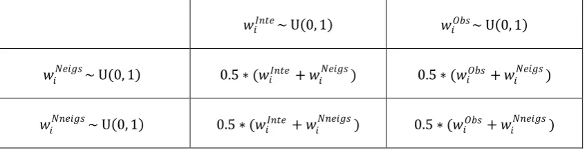
observations. All of an agent‟s four weights are randomly chosen from uniform distribution on range [0, 1) and do not change across time. The weights of four kinds of information sources in trust-updating is four linear combinations of either 𝑤𝑖𝑁𝑒𝑖𝑔𝑠 or 𝑤𝑖𝑁𝑛𝑒𝑖𝑔𝑠and either 𝑤𝑖𝐼𝑛𝑡𝑒 or 𝑤𝑖𝑂𝑏𝑠.1 That is, the weight of interacting with neighbors in ai‟s trust-updating is a linear
combination of 𝑤𝑖𝑁𝑒𝑖𝑔𝑠 and 𝑤𝑖𝐼𝑛𝑡𝑒; the weight of interacting with non-neighbors in ai‟s
trust-updating is a linear combination of 𝑤𝑖𝑁𝑛𝑒𝑖𝑔𝑠 and 𝑤𝑖𝐼𝑛𝑡𝑒;the weight of observing interactions between two mutual neighbors in ai‟s trust-updating is a linear combination of 𝑤𝑖𝑁𝑒𝑖𝑔𝑠 and 𝑤𝑖𝑂𝑏𝑠;
the weight of observing interactions between two mutual non-neighbors in ai‟s trust-updating is a
[image:9.595.89.514.497.606.2]linear combination of 𝑤𝑖𝑁𝑛𝑒𝑖𝑔𝑠 and 𝑤𝑖𝑂𝑏𝑠. Specifically, we set the weights of four kinds of information sources as follows (see Table 2.3-1):
Table 2.3-1 Weights of four kinds of information sources in ai‟s trust-updating
𝑤𝑖𝐼𝑛𝑡𝑒~ U 0, 1 𝑤
𝑖𝑂𝑏𝑠~ U 0, 1
𝑤𝑖𝑁𝑒𝑖𝑔𝑠~ U 0, 1 0.5∗(𝑤𝑖𝐼𝑛𝑡𝑒 +𝑤𝑖𝑁𝑒𝑖𝑔𝑠) 0.5∗(𝑤𝑖𝑂𝑏𝑠 +𝑤𝑖𝑁𝑒𝑖𝑔𝑠)
𝑤𝑖𝑁𝑛𝑒𝑖𝑔𝑠~ U 0, 1 0.5∗(𝑤𝑖𝐼𝑛𝑡𝑒 +𝑤𝑖𝑁𝑛𝑒𝑖𝑔𝑠) 0.5∗(𝑤𝑖𝑂𝑏𝑠+𝑤𝑖𝑁𝑛𝑒𝑖𝑔𝑠)
2.3.5 Initialization of unilateral link weights
Unilateral link weights are what an agent, say ai, depends on to actively choose a neighbor as a
potential interaction partner when his scope of choosing is within neighborhood, and unilateral link weights do not change within a time period. The neighbor to whom ai assigns larger unilateral
link weight is with higher probability to be chosen. Let LWi,t be the set of unilateral link weights
that ai holds for all his neighbors in time period t. We set
𝐿𝑊𝑖,𝑡 = {𝑙𝑤𝑖𝑗,𝑡|𝑎𝑗 ∈ 𝑁𝑒𝑖𝑔𝑖, 0≤ 𝑙𝑤𝑖𝑗,𝑡 ≤1 and 𝑙𝑤𝑗 𝑖𝑗,𝑡 = 1}
1 Here an implicit assumption is that 𝑤
9
and set
𝑝𝑖𝑗𝐴𝑃𝐼,𝑡,𝜏 =𝑙𝑤𝑖𝑗,𝑡 (0≤ 𝜏 ≤ 𝑅𝑒𝑞𝑖𝐼𝑛𝑡𝑒,𝑡 and 𝜏ϵN+)
Therein, lwij,t the unilateral link weight that ai assigns to his neighbor aj in time period t. It equals
𝑝𝑖𝑗𝐴𝑃𝐼,𝑡,𝜏, the probability that ai actively chooses his arbitrary neighbor aj as a potential interaction
partner when neighborhood is ai‟s choosing scope in sub-time period 𝜏 of time period t. Note that
𝑙𝑤𝑖𝑗,𝑡 ≠ 𝑙𝑤𝑗𝑖,𝑡, since the network structure is a directed weighted graph in this paper, as aforementioned.
Initially, an agent‟s unilateral link weights follow discrete uniform distribution, which means that
in the first time period, each neighbor of ai is with probability
1
𝑁𝑢𝑚𝑖𝑁𝑒𝑖𝑔𝑠 (𝑁𝑢𝑚𝑖
𝑁𝑒𝑖𝑔𝑠is the number
of ai‟s neighbors) to be chosen as a potential interaction partner by ai. That is, initially,
𝑝𝑖𝑗𝐴𝑃𝐼,𝑡=1,𝜏 = P 𝑃𝑎𝑟𝑡𝑛𝑒𝑟𝑖𝐴𝑃𝐼,𝑡=1,𝜏 =𝑎𝑗|𝑃𝑇𝑖𝐴𝑃𝐼,𝑡=1,𝜏 = 0 =
1
𝑁𝑢𝑚𝑖𝑁𝑒𝑖𝑔𝑠 (𝑎𝑗 ∈ 𝑁𝑒𝑖𝑔𝑠𝑖; 0≤ 𝜏 ≤ 𝑅𝑒𝑞𝑖𝐼𝑛𝑡𝑒,𝑡 and 𝜏ϵN+)
𝑃𝑎𝑟𝑡𝑛𝑒𝑟𝑖𝐴𝑃𝐼,𝑡=1,𝜏 represents the partner that ai actively chooses as his potential interaction partner in
sub-time period 𝜏 of time period t=1. 𝑃𝑇𝑖𝐴𝑃𝐼,𝑡=1,𝜏 = 0 represents the condition that the partner type of the chosen potential interaction partner is a neighbor (“neighbors” is represented by 0 and “non-neighbors” by 1). The specific mechanism agents update their unilateral link weights for the next time period when a time period ends will be introduced in detail in section 2.4.3.
2.4 Micro-level process
Each time period contains 𝜏=𝑅𝑒𝑞𝑖𝐼𝑛𝑡𝑒,𝑡 sub-time periods (𝑅𝑒𝑞𝑖𝐼𝑛𝑡𝑒,𝑡 = 20 in this paper). The micro-level process in each time period contains three main tasks: 1) all agents one by one have an opportunity to actively make an interaction request (described in 2.4.1), and this rotation repeats for 𝑅𝑒𝑞𝑖𝐼𝑛𝑡𝑒,𝑡 times; 2) all agents one by one update their trustworthiness (namely probability to cooperate in each actual interaction) for the next time period (described in 2.4.2); 3) all agents one by one modify their unilateral link weights for the next time period (described in 2.4.3).
2.4.1 Interaction, information diffusion and trust-updating
1) Interaction decision for active potential interactions
For each sub-period𝜏 (𝜏 ∈N+ and 𝜏 ≤ 𝑅𝑒𝑞𝑖𝐼𝑛𝑡𝑒,𝑡 ) in time step t, every agent, in turn in a shuffled order, has an opportunity to actively make an interaction request to others. Whether an agent will grasp the opportunity and enter the next step of choosing a potential interaction partner is determined by his willingness to interact, namely his own trust in this paper. That is, ai with a
probability equal to his trust continues to choose a potential interaction partner.
10
𝑁𝑢𝑚𝑖𝑃𝐼,𝑡 =𝑁𝑢𝑚𝑖𝑃𝐼,𝑡
,𝑁+𝑁𝑢𝑚
𝑖,𝑡
𝑃𝐼,𝑁𝑛
𝑁𝑢𝑚𝑖𝑃𝐼,𝑡 represents ai‟s number of potential interactions within time period t. 𝑁𝑢𝑚𝑖𝑃𝐼,𝑡,𝑁represents
ai‟s number of potential interactions with his neighbors in time period t. 𝑁𝑢𝑚𝑃𝐼𝑖,𝑡,𝑁𝑛 represents ai‟s
number of potential interactions with his non-neighbors in time period t.
However, as we notice, an agent‟s number of potential interactions also equals his active interaction requests and interaction requests from others (passive interactions).Thus, the second way to calculate an agent‟s number of potential interactions within time period t is:
𝑁𝑢𝑚𝑃𝐼𝑖,𝑡 =𝑁𝑢𝑚𝑖𝐴𝑃𝐼,𝑡 +𝑁𝑢𝑚𝑃𝑃𝐼𝑖,𝑡 =𝑅𝑒𝑞𝑖𝐼𝑛𝑡𝑒,𝑡 +𝑁𝑢𝑚𝑖𝑃𝑃𝐼,𝑡
𝑁𝑢𝑚𝑖𝐴𝑃𝐼,𝑡 represents ai‟s number of active potential interactions in time period t. 𝑁𝑢𝑚𝑖𝑃𝑃𝐼,𝑡
represents ai‟s number of passive potential interactions in time period t.According to the setting in
this paper, 𝑁𝑢𝑚𝑖𝐴𝑃𝐼,𝑡 =𝑅𝑒𝑞𝑖𝐼𝑛𝑡𝑒,𝑡 = 20.
2) To choose a potential interaction partner
Following Macy and Skvoretz (1998), in this paper the degree of embeddedness in social network is also assumed. Degree of embededness in social network, as a parameter, is represented by a float number in range [0, 1). When aiis going to actively propose an interaction request, his
potential interaction partner will be chosen either from his neighborhood with probability equal to degree of embeddedness in social network or from his non-neighborhood with probability equal to 1 minus degree of embeddedness in social network.1
If ai‟s potential interaction partner is definitely going to be chosen from neighborhood, which
neighbor on earth will be chosen hinges on ai‟s unilateral link weights assigned to his neighbors.
On contrast, if ai‟s potential interaction partner is definitely outside his neighborhood, a
non-neighbor will be randomly chosen among ai‟s non-neighbors with equal likelihood. That is,
𝑝𝑖𝑗𝑃𝐼,𝑡,𝜏 =
𝑙𝑤𝑖𝑗,𝑡 if 𝑎𝑗 ∈ 𝑁𝑒𝑖𝑔𝑠𝑖
1
𝑁𝑢𝑚𝑖𝑁𝑛𝑒𝑖𝑔𝑠 if 𝑎𝑗 ∈ 𝑁𝑒𝑖𝑔𝑠𝑖
𝐶
𝑝𝑖𝑗𝑃𝐼,𝑡,𝜏 represents the probability that aichooses aj as his potential interaction partner in sub-time
period 𝜏 of time period t. If ajbelongs to ai‟s neighbors, the probability that aj is chosen is 𝑙𝑤𝑖𝑗,𝑡;
if aj belongs to ai‟s non-neighbors, the probability is
1
𝑁𝑢𝑚𝑖𝑁𝑛𝑒𝑖𝑔𝑠. 𝑁𝑢𝑚𝑖
𝑁𝑛𝑒𝑖𝑔𝑠 is the number of a
i‟s
non-neighbors. If the former (𝑎𝑗 ∈ 𝑁𝑒𝑖𝑔𝑠𝑖), aj‟s number of passive potential interactions (namely,
passive potential interactions) from neighbors in the current time period increases by 1.2 Namely,
𝑁𝑢𝑚𝑗𝑃𝑃𝐼,𝑡
,𝑁 ← 𝑁𝑢𝑚
𝑗𝑃𝑃𝐼,𝑡
,𝑁+ 1 if 𝑎
𝑗 ∈ 𝑁𝑒𝑖𝑔𝑠𝑖
1 “Degree of embededness in social network” here only represents the probability that an agent encounters a
neighbor in a potential interaction; it does not represent an agent‟s subjective willingness to interact with a
neighbor.
11
Number of passive potential interactions from neighbors is counted for trustworthiness updating in 2.4.2. Whether ai‟s chosen potential interaction partner aj (either a neighbor or a non-neighbor)
would like to participate in the interaction then depends on ajwillingness to interact determined by
aj‟s own trust. Only if aj agrees to interact, the interaction will actually happen, and ai and aj enter
the next step of strategy decision; otherwise, the actual interaction won‟t happen.
3) Pure strategy decision
Applying which pure strategy for the forthcoming actual interaction is determined by the agents‟ probability of cooperation, namely their own trustworthiness in this paper. If a random number chosen from uniform distribution in range [0, 1) is smaller than an agent‟s trustworthiness (probability to cooperate), his strategy will be “Cooperate”; otherwise, his strategy will be “Defect”. Hence, each agent is actually using a mixed strategy. That is,
𝑃𝑆𝑖← 0 if 𝑟𝑖
𝑠𝑡𝑟𝑎 ∈[0,𝑇𝑟𝑤 𝑖,𝑡]
1 if 𝑟𝑖𝑠𝑡𝑟𝑎 ∈(𝑇𝑟𝑤𝑖,𝑡, 1)
𝑃𝑆𝑖represents the pure strategy that agent aiwould use in a forthcoming actual interaction. “0”
represents “Cooperation” and “1” “Defection”. 𝑟𝑖𝑠𝑡𝑟𝑎 is a pseudo number following uniform distribution in range [0, 1). 𝑇𝑟𝑤𝑖,𝑡 is agent ai‟s trustworthiness in time period t.
4) Payoff matrix mutation
The actual interaction process is modeled by non-cooperative and symmetric prisoners‟ dilemmas. Denote matrix Ag as a general form of payoff matrixes of prisoners‟ dilemma and set
𝑨𝑔 = 𝑎11 𝑎12
𝑎21 𝑎22
a11 is an agent‟s payoff when both he and his partner apply strategy “Cooperation”; a12 is an
agent‟s payoff when he alone uses strategy “Cooperation” while his partner uese strategy “Defect”; a21 is an agent‟s payoff when he plays strategy “Defect” and his partner plays strategy
“Cooperation”; a22is an agent‟s payoff when both players apply strategy “Defect”. Then, the
elements of payoff matrix Ag should satisfy 𝑎21 > 𝑎11 > 𝑎22 > 𝑎12 and 𝑎11 > 𝑎21+ 𝑎12
2 for a
game to be a prisoners‟ dilemma.
What is more important for trust-updating later in this paper, we define marginal rate of exploitation (MRE) of a given payoff matrix Ag as
𝑀𝑅𝐸Ag ,𝐶/𝐷 =𝑎11 − 𝑎12 𝑎21 − 𝑎11
𝑀𝑅𝐸𝐴𝑔,𝐶/𝐷 represents marginal rate of exploitation of pure strategy “Defection” to pure strategy
“Cooperation” under payoff matrix Ag. It measures how much a defector can gain from deviating one unit of payoff from pure strategy “Cooperation” on the loss of his game partner who is a cooperator. MRE is positive.
12
𝑨= 𝑎11
𝐴 𝑎12𝐴
𝑎21𝐴 𝑎22𝐴 and 𝑨𝑚𝑢𝑡 = 𝑎11
𝐴𝑚𝑢𝑡 𝑎12𝐴𝑚𝑢𝑡
𝑎21𝐴𝑚𝑢𝑡 𝑎22𝐴𝑚𝑢𝑡
Therein, Amut is a mutated version of A. Thus, the marginal rate of exploitation of payoff matrix A
is:
𝑀𝑅𝐸𝐴,𝐶/𝐷=𝑎11𝐴 − 𝑎12𝐴 𝑎21𝐴 − 𝑎11𝐴
Besides the general conditions a prisoners‟ dilemma should satisfy, A and Amut in this paper also satisfy 𝑎11𝐴𝑚𝑢𝑡 =𝑎11𝐴, 𝑎22𝐴𝑚𝑢𝑡 =𝑎22𝐴 , 𝑎21𝐴𝑚𝑢𝑡 >𝑎21𝐴 and 𝑎12𝐴𝑚𝑢𝑡 <𝑎12𝐴 to ensure that the mutated payoff matrix Amut enlarges the exploitation degree of unilateral defection compared to the original payoff matrix A, and to have comparability as well. At the same time, we denote relative exploitation degree (RED) of payoff matrix Amut over A as
𝑅𝐸𝐷𝐴𝑚𝑢𝑡/𝐴 = 𝑎21𝐴𝑚𝑢𝑡 − 𝑎12𝐴𝑚𝑢𝑡
𝑎21𝐴 − 𝑎12𝐴
Relative exploitation degree is constructed to measure to which degree a mutated payoff matrix
Amut enlarges the interest conflict of the original payoff matrix A. Both marginal rate of exploitation and relative exploitation degree are for trust updating in 6) in 2.4.1. Numerically, A=
3 1
4 2 in this paper and A
mut
is a parameter with different candidate values. For example, when
Amut = 3 0
5 2 , we get
𝑀𝑅𝐸𝐴,𝐶/𝐷 =𝑎11𝐴 − 𝑎12𝐴 𝑎21𝐴 − 𝑎11𝐴 =
3−1
4−3= 2
𝑅𝐸𝐷𝐴𝑚𝑢𝑡/𝐴 = 𝑎21𝐴𝑚𝑢𝑡 − 𝑎12𝐴𝑚𝑢𝑡 𝑎21𝐴 − 𝑎12𝐴 =
5−0
4−1=
5 3
Payoff matrix decision comes after pure strategy decision. The initiator (the active interaction party) of a potential interaction has an exclusive right to unilaterally change payoff matrix from A
to Amut with probability pAmut which is a parameter in this paper, on condition that the initiator has already decided to apply “Defection” for this forthcoming actual interaction.1 As long as no payoff matrix mutation happens, the interaction will carry on with the original payoff matrix A. That is,
𝑃𝑀𝑖,𝑡,𝜏 = 𝐴
if 𝑟𝑃𝑀 ∈[0,𝑝𝐴𝑚𝑢𝑡]
𝐴𝑚𝑢𝑡 if 𝑟𝑃𝑀 ∈(𝑝𝐴𝑚𝑢𝑡, 1)
𝑃𝑀𝑖,𝑡,𝜏 represents ai‟s payoff matrix decision for his active potential interaction in sub-time period
𝜏 in time period t. 𝑟𝑃𝑀is a pseudo random number. Due to the specific conditions that A and Amut
should satisfy in this paper, we suppose that when active actor chooses Amut: 1) the passive actor cannot discover he is under Amut unless the passive actor plays “Cooperation”; 2) observers cannot
1 Even though mutation probability is very small in nature (e.g., Seltzer and Smirnov, 2015), it is not set that small
13
either detect their observed interaction is under Amut unless the observed interaction is unilateral defect.
5) To play the game
After pure strategies and payoff matrix for the forthcoming interaction have been decided, the two interaction parties begin to play the game. What each of both interacting parties should record through each actual interaction in a current time period is two aspects: i) counting his own actual interactions (including both active ones and passive ones) and “Cooperation” (no matter what pure strategy his partner uses) no matter whether his partner is a neighbor or a non-neighbor; ii) counting actual interactions happening with each of his neighbors and “Cooperation” that each of his neighbors applies to him according to his neighbors‟ identity. All these are reset to zero at the beginning of every time period (not sub-time period). Therein, i) is for trustworthiness updating in 2.4.2; ii) is for unilateral link weights updating in 2.4.3.
Formally, in each actual interaction, for purpose of i),
𝑁𝑢𝑚𝑖𝐴𝐼,𝑡 ← 𝑁𝑢𝑚𝑖𝐴𝐼,𝑡 + 1
𝑁𝑢𝑚𝑖𝐶,𝑡 ← 𝑁𝑢𝑚𝑖𝐶,𝑡+ 1 if 𝑃𝑆𝑖= 0
𝑁𝑢𝑚𝑖𝐴𝐼,𝑡 represents the times of ai‟s actual interactions in time period t. 𝑁𝑢𝑚𝑖𝐶,𝑡 represents the
times that ai uses “Cooperation” in time period t. For purpose of ii),
𝑁𝑢𝑚𝑖𝑗𝐴𝐼,𝑡 ← 𝑁𝑢𝑚𝑖𝑗𝐴𝐼,𝑡 + 1 if 𝑎𝑗 ∈ 𝑁𝑒𝑖𝑔𝑠𝑖
𝑁𝑢𝑚𝑖𝑗,𝑡
𝐶𝑗 ← 𝑁𝑢𝑚
𝑖𝑗,𝑡 𝐶𝑗
+ 1 if 𝑎𝑗 ∈ 𝑁𝑒𝑖𝑔𝑠𝑖 and 𝑃𝑆𝑗 = 0
𝑁𝑢𝑚𝑖𝑗𝐴𝐼,𝑡 represents the times of ai‟s actual interactions with his neighbor aj in time period t.
𝑁𝑢𝑚𝑖𝑗𝐶𝑗,𝑡 represents the times that his neighbor a
j applies “Cooperation” to ai in time period t.
6) Diffusion of interaction information (Observed by others)
It is possible that others who are not interacting parties get informed of the situation and result of an interaction. Except the two interaction parties, say aiand aj, the agents in the artificial society
are separated into two sets: one is the union-neighbor set UNeigij in which the agents are
neighbors of either of the interaction parties; the other is set DNeigij in which agents are neighbors
of neither of the interaction parties. Thus, when the interaction parties aiand aj are mutual
neighbors,
𝑈𝑁𝑒𝑖𝑔𝑖𝑗 =𝑁𝑒𝑖𝑔𝑖∪ 𝑁𝑒𝑖𝑔𝑗−{𝑎𝑖,𝑎𝑗}
𝐷𝑁𝑒𝑖𝑔𝑖𝑗 =𝑁 −(𝑁𝑒𝑖𝑔𝑖∪ 𝑁𝑒𝑖𝑔𝑗)
When the interaction parties aiand aj are mutual non-neighbors,
14
𝐷𝑁𝑒𝑖𝑔𝑖𝑗 =𝑁 − 𝑁𝑒𝑖𝑔𝑖∪ 𝑁𝑒𝑖𝑔𝑗 −{𝑎𝑖,𝑎𝑗}
The probability that the interaction information of aiand aj diffuses in these two interacting parties‟
neighborhoods UNeigi,j is p IDN
, and the probability diffusing in their non-neighborhoods DNeigi,j is
pIDNn. Both pIDNand pIDNnare random numbers following uniform distribution in range [0,1) and act as parameters whose influence will be investigated under four different candidate values.
Then, the interaction information of aiand aj starts “diffusing” separately in UNeigi,j and DNeigi,j.
Whether an outside agent ak (an agent who is not one of the interacting parties) will get informed
of the just happening interaction depends on whether he belongs to UNeigi,j or DNeigi,j, and his
own probability of information acquisition from neighbors 𝑝𝑘𝐼𝐴𝑁 and from non-neighbors 𝑝𝑘𝐼𝐴𝑁𝑛. That is,
𝑝𝑘𝐺𝐼= 𝑝𝑘
𝐼𝐴𝑁 if 𝑎
𝑘 ∈ 𝑈𝑁𝑒𝑖𝑔𝑖𝑗
𝑝𝑘𝐼𝐴𝑁𝑛 if 𝑎𝑘 ∈ 𝐷𝑁𝑒𝑖𝑔𝑖𝑗
𝑝𝑘𝐺𝐼 is the probability that an outsider ak gets informed of a piece of interaction information
between ai and aj. What an observing agent will get informed about others‟ interaction is 1) the
strategy combination, that is whether the observed interaction is “mutual cooperation”, “unilateral defection” or “mutual defection”;2) the relationship between the observed interacting parties, namely “mutual neighbors” or “mutual non-neighbors” and 3) the specific payoff matrix, that is whether the payoff matrix is a mutated one. Note that Amut can only manifest itself in the situation of unilateral defection because Amut has the same values with A in situations of “mutual cooperation” and “mutual defection” according to the settings in this paper.
7) To update self‟s trust
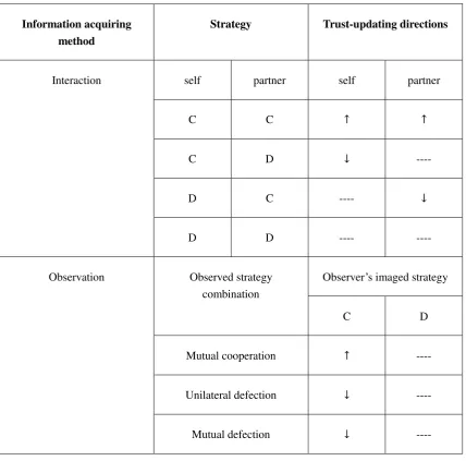
i) Trust-updating directions (qualitative trust-updating)
Changes of trust have three directions: increase, decrease and remain unchanged. In order to clarity how trust changes and when, it is necessary for us to at first distinguish trust-increasing events, trust-destroying events and trust-invariant events. This is analyzed from two angles: interacting agents and observing agents.
·Interacting agents
For the two interacting agents, in the situation of mutual cooperation, both agents‟ trust increase; in the situation of unilateral defection, the cooperative agent‟s trust decreases while the defective agent‟s trust remains unchanged; in the situation of mutual defection, both agents‟ trust keeps invariant. (Also see Table 2.4-1)
·Observing agents
15
[image:16.595.85.514.120.543.2]will not change. (Also see Table 2.4-1)
Table 2.4-1 Trust-updating directions
Information acquiring
method
Strategy Trust-updating directions
Interaction self partner self partner
C C ↑ ↑
C D ↓ ----
D C ---- ↓
D D ---- ----
Observation Observed strategy
combination
Observer‟s imaged strategy
C D
Mutual cooperation ↑ ----
Unilateral defection ↓ ----
Mutual defection ↓ ----
ii) Quantitative trust-updating
Quantitative trust-updating is based on a certain amount ∆𝑇𝑟𝐵𝑎𝑠𝑒 which equals 0.05. How much exactly an agent will update his trust hinges on 1) marginal rate of exploitation of payoff matrix A
(namely, 𝑀𝑅𝐸A,𝐶/𝐷), 2) relative exploitation degree of Amut
compared to A (namely, 𝑅𝐸𝐷𝐴𝑚𝑢𝑡/𝐴), and 3) ai‟s own weights for four kinds of information sources (the four possible combinations of
either 𝑤𝑖𝑁𝑒𝑖𝑔𝑠or 𝑤𝑖𝑁𝑛𝑒𝑖𝑔𝑠 and either 𝑤𝑖𝐼𝑛𝑡𝑒or 𝑤𝑖𝑂𝑏𝑠 shown in Table 2.3-1).
·Interacting agents
Assume ai interacts with his neighbor aj. If both ai and aj apply “Cooperation”,
𝑇𝑟𝑖 ←min(𝑇𝑟𝑖+ 0.5∗ 𝑤𝑖𝑁𝑒𝑖𝑔𝑠+𝑤𝑖𝐼𝑛𝑡𝑒 ∗ ∆𝑇𝑟𝐵𝑎𝑠𝑒, 1)
16
𝑇𝑟𝑖 ←max(𝑇𝑟𝑖−0.5∗ 𝑀𝑅𝐸𝐴,𝐶/𝐷∗ 𝑤𝑖𝑁𝑒𝑖𝑔𝑠+𝑤𝑖𝐼𝑛𝑡𝑒 ∗ ∆𝑇𝑟𝐵𝑎𝑠𝑒, 0)
If ai unilaterally uses “Cooperation” under payoff matrix A mut
,
𝑇𝑟𝑖←max(𝑇𝑟𝑖−0.5∗ 𝑅𝐸𝐷𝐴𝑚𝑢𝑡/𝐴∗ 𝑀𝑅𝐸𝐴,𝐶/𝐷∗ 𝑤𝑖𝑁𝑒𝑖𝑔𝑠 +𝑤𝑖𝐼𝑛𝑡𝑒 ∗ ∆𝑇𝑟𝐵𝑎𝑠𝑒, 0)
When ai‟s interaction partner is a non-neighbor aj, 𝑤𝑖𝑁𝑛𝑒𝑖𝑔𝑠 should replace 𝑤𝑖𝑁𝑒𝑖𝑔𝑠. At the same
time, aj should also update his trust according to the same rule.
·Observing agents
Assume ak observes the interaction between two mutual neighbors ai and aj. If both ai and aj apply
“Cooperation” and ak‟s imaged pure strategy is also “Cooperation”,
𝑇𝑟𝑘 ←min(𝑇𝑟𝑘+ 0.5∗ 𝑤𝑘𝑁𝑒𝑖𝑔𝑠 +𝑤𝑘𝑂𝑏𝑠 ∗ ∆𝑇𝑟𝐵𝑎𝑠𝑒, 1)
If not both ai and aj apply “Cooperation”, when ak‟s imaged pure strategy is “Cooperation” and the
observed payoff matrix is not Amut,
𝑇𝑟𝑘 ←max(𝑇𝑟𝑘−0.5∗ 𝑀𝑅𝐸𝐴,𝐶/𝐷∗ 𝑤𝑘𝑁𝑒𝑖𝑔𝑠 +𝑤𝑘𝑂𝑏𝑠 ∗ ∆𝑇𝑟𝐵𝑎𝑠𝑒, 0)
If not both ai and aj apply “Cooperation”, when ak‟s imaged pure strategy is “Cooperation” but the
observed payoff matrix is Amut,
𝑇𝑟𝑘 ←max(𝑇𝑟𝑘−0.5∗ 𝑅𝐸𝐷𝐴𝑚𝑢𝑡/𝐴∗ 𝑀𝑅𝐸𝐴,𝐶/𝐷∗ 𝑤𝑘𝑁𝑒𝑖𝑔𝑠 +𝑤𝑘𝑂𝑏𝑠 ∗ ∆𝑇𝑟𝐵𝑎𝑠𝑒, 0)
When ak observes an interaction happening between two mutual non-neighbors, 𝑤𝑘𝑁𝑛𝑒𝑖𝑔𝑠 should
replace 𝑤𝑘𝑁𝑒𝑖𝑔𝑠.
2.4.2 To update self‟s trustworthiness
Agents‟ updating of their own trustworthiness (namely their probability of cooperation in an interaction) is considered as a process of strategy learning. We constrain the objects of an agent‟s strategy-learning within his neighbors. Every agent updates his trustworthiness near the end of a time period. What needs to be done for an agent ai is searching out his neighbor, say 𝑎𝑗0, with
highest number of passive potential interactions 𝑁𝑢𝑚𝑗
0,𝑡
𝑃𝑃𝐼,𝑁 in the current time period. If
𝑁𝑢𝑚𝑗0,𝑡
𝑃𝑃𝐼,𝑁 is larger than a
i‟s own times of passive potential interactions 𝑁𝑢𝑚𝑖𝑃𝑃𝐼,𝑡 ,𝑁, ai would
switch his trustworthiness to 𝑎𝑗0‟s cooperation rate of 𝑅𝑗𝐶0,𝑡 in the current time period t and take it as his (mixed) strategy for the next time period; otherwise, ai would maintain his current
trustworthiness over to the next time period. The reason why the base of strategy learning is set at agents‟ cooperation rate of a current time period t rather than agents‟ probability of cooperation in an interaction is that it is assumed that an agent‟s probability of cooperation in an interaction is not observable for other agents while his cooperation rate is, on contrast.
Formally, let Neigirepresent the set of ai‟s neighbor set in which his strategy-learning candidates
are in time period t and ajbe an arbitrary element in Neigi. The agent aj0 with the highest number
17
𝑗0= argmax𝑗 𝑗 𝑁𝑢𝑚𝑗𝑃𝑃𝐼,𝑡 ,𝑁,𝑎𝑗 ∈ 𝑁𝑒𝑖𝑔𝑖}
Thus,
𝑇𝑟𝑤𝑖,𝑡+1= 𝑅𝑗0,𝑡
𝐶 if 𝑁𝑢𝑚
𝑗0,𝑡
𝑃𝑃𝐼,𝑁 > 𝑁𝑢𝑚
𝑖,𝑡
𝑃𝑃𝐼,𝑁 𝑇𝑟𝑤𝑖,𝑡 otherwise
Therein
𝑅𝑗0,𝑡
𝐶 = 𝑁𝑢𝑚𝑗0,𝑡
𝐶
𝑁𝑢𝑚𝑗𝐴𝐼0,𝑡
𝑁𝑢𝑚𝑗𝐴𝐼0,𝑡 ≠0 1
𝑅𝑗0,𝑡
𝐶 represents agent j
0‟s cooperation rate in time period t, 𝑁𝑢𝑚𝑗𝐶0,𝑡 represents agent j0‟s total
times of cooperation in time period t and 𝑁𝑢𝑚𝑗𝐴𝐼0,𝑡 represents agent j0‟s total times of actual (not
potential) interactions in time period t.
2.4.3 To update self‟s unilateral link weights
At the end of each time step t, each agent updates his unilateral link weights for the next time step t+1. At first, ai evaluates each of his neighbor‟s cooperation rates only to him according to
𝑅𝑖𝑗,𝑡
𝐶𝑗 = 𝑁𝑢𝑚𝑖𝑗,𝑡
𝐶𝑗
𝑁𝑢𝑚𝑖𝑗𝐴𝐼,𝑡
(𝑁𝑢𝑚𝑖𝑗𝐴𝐼,𝑡 ≠0)
0.2 (𝑁𝑢𝑚𝑖𝑗𝐴𝐼,𝑡 = 0)
(𝑎𝑗 ∈ 𝑁𝑒𝑖𝑔𝑠𝑖)
𝑅𝑖𝑗𝐶𝑗,𝑡 represents a
i‟s evaluation on his arbitrary neighbor aj‟s cooperation rate to him in the end of
time period t. 𝑁𝑢𝑚𝑖𝑗𝐶𝑗,𝑡 is the times that ai‟s neighbor aj applies “Cooperation” to aiin time period
t. 𝑁𝑢𝑚𝑖𝑗𝐴𝐼,𝑡 is the times of ai‟s actual interactions with his neighbor aj in time period t. (𝑁𝑢𝑚𝑖𝑗,𝑡
𝐶𝑗
and 𝑁𝑢𝑚𝑖𝑗𝐴𝐼,𝑡 have been introduced in 5) in 2.4.1.) 𝑁𝑢𝑚𝑖𝑁𝑒𝑖𝑔𝑠 is ai‟s number of neighbors. 0.2 is
used as a proxy of 𝑅𝑖𝑗𝐶𝑗,𝑡 whenever ai has no actual interaction records of his neighbor aj in time
period t.
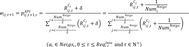
Then ai updates his link weights for the next time period t+1 according to the mechanism below:
1 𝑁𝑢𝑚
𝑗0,𝑡
𝐴𝐼 will be definitely larger than 0 if 𝑁𝑢𝑚 𝑗0,𝑡
𝑃𝑃𝐼,𝑁> 𝑁𝑢𝑚 𝑖,𝑡
𝑃𝑃𝐼,𝑁, since the lower limit of an arbitrary agent‟s
18
𝑙𝑤𝑖𝑗,𝑡+1=𝑝𝑖𝑗𝐴𝑃𝐼,𝑡+1,𝜏 =
𝑅𝑖𝑗𝐶𝑗,𝑡+𝛿
𝑅𝑖𝑗,𝑡 𝐶𝑗
+𝛿
𝑖+𝑁𝑢𝑚𝑖
𝑁𝑒𝑖𝑔𝑠
2
𝑗=𝑖−𝑁𝑢𝑚𝑖
𝑁𝑒𝑖𝑔𝑠
2
=
𝑅𝑖𝑗𝐶𝑗,𝑡+ 1
𝑁𝑢𝑚𝑖𝑁𝑒𝑖𝑔𝑠
𝑅𝑖𝑗,𝑡 𝐶𝑗
+ 1
𝑁𝑢𝑚𝑖𝑁𝑒𝑖𝑔𝑠
𝑖+𝑁𝑢𝑚𝑖
𝑁𝑒𝑖𝑔𝑠
2
𝑗=𝑖−𝑁𝑢𝑚𝑖
𝑁𝑒𝑖𝑔𝑠
2
(𝑎𝑗 ∈ 𝑁𝑒𝑖𝑔𝑠𝑖, 0≤ 𝜏 ≤ 𝑅𝑒𝑞𝑖𝐼𝑛𝑡𝑒,𝑡 and 𝜏 ∈N+)
𝑙𝑤𝑖𝑗,𝑡+1 represents the unilateral link weight that ai assigns to his neighbor aj for the next time
period. 𝑝𝑖𝑗𝐴𝑃𝐼,𝑡+1,𝜏 represents the probability that ai actively chooses his neighbor 𝑎𝑗 as his
potential interaction partner when ai should choose an potential interaction partner within his
neighborhood in any sub-time period 𝜏 of time period t+1. What is more, we define 𝛿 as relationship maintenance strength which is a constant and used for: 1) controlling to which degree a relationship is maintained over to the next time period even if an agent‟s neighbor defects in all actual interaction between them in the current time period; 2) and at the same time for an agent to attach enough importance on neighbors‟ cooperation rate in the actual interactions between them in the current time period. The link-weights updating rule is created like this because embeddedness in social network is an interested parameter in this paper and, hence, it is undesirable to totally delete any relationship forever. In this paper, we set 𝛿=𝑙𝑤𝑖𝑗,𝑡=1=
1
𝑁𝑢𝑚𝑖𝑁𝑒𝑖𝑔𝑠, namely ai‟s initial unilateral link weight to his arbitrary neighbor aj, in order to keep
consistence with the fact that, generally, a neighbor is with less probability to be chosen in a larger neighborhood
3 Results and analysis
Simulations are constrained within an artificial society of 100 agents and with an original payoff
matrix of 3 1
4 2 , and focus on the influence of seven parameters, namely number of immediate
[image:19.595.111.486.79.173.2]neighbors, degree of embededness in social network, mutation probability of payoff structure, mutated payoff matrix, proportion of individuals with high trust in population, probability of information diffusion in neighbors and probability of information diffusion in non-neighbors. The candidate values of each parameter of interest are listed in Table 3-1:1
Table 3-1: Candidate values of each parameter of interest
Parameters Candidate values
1) Population size (ps) 100
2) Number of immediate neighbors (nn) 4, 6, 8, 10
1 The abbreviations of these terms in section 3 are not the same as the mathematical symbols in section 2. The
19
3) Degree of embededness in social network (se)
0.6, 0.7, 0.8, 0.9
4) Mutation probability of payoff structure (mpps)
0.1, 0.2, 0.3, 0.4
5) Original payoff matrix (A) 3 1
4 2
6) Mutated payoff matrix (Amut) 3 0
5 2 ,
3 −1
6 2 ,
3 −2
7 2 ,
3 −3
8 2
7) Proportion of individuals with high trust in population (pht)
0.6, 0.7, 0.8, 0.9
8) Probability of information diffusion in neighbors (pidn)
0.6, 0.7, 0.8, 0.9
9) probability of information diffusion in non-neighbors (pidnn)
0.1, 0.2, 0.3, 0.4
Note: Numbers or matrixes with a short horizontal line underneath are the parameter values used in base-line simulation.
For every parameter value portfolio under investigation, we are interested in the evolution of two variables: person-time of interaction and person-time of cooperation. Person-time, in this paper, is the sum of every individual‟s number of some record (such as, actual interaction and cooperation) in a time period. Formally,
𝑃𝑒𝑟𝑠𝑜𝑛𝑇𝑖𝑚𝑒𝑡𝐴𝐼= 𝑁𝑢𝑚𝑖𝐴𝐼,𝑡
100
𝑖=1
𝑃𝑒𝑟𝑠𝑜𝑛𝑇𝑖𝑚𝑒𝑡𝐶= 𝑁𝑢𝑚𝑖𝐶,𝑡 100
𝑖=1
𝑃𝑒𝑟𝑠𝑜𝑛𝑇𝑖𝑚𝑒𝑡𝐴𝐼 is the person-time of actual interactions within time period t which equals the
20
4000].1 “Person-time” is adopted because multiple interactions within a time period are allowed for each agent and every agent is actually using a mixed strategy rather than a fixed pure strategy in a time period, and additionally, it is the impact of interaction information that is important for both interacting agents and observing agents.
Since there are very large potential combinations of parameter values, we will explore the influence of each parameter of interest based on a base-line simulation.
3.1 Base-line simulation
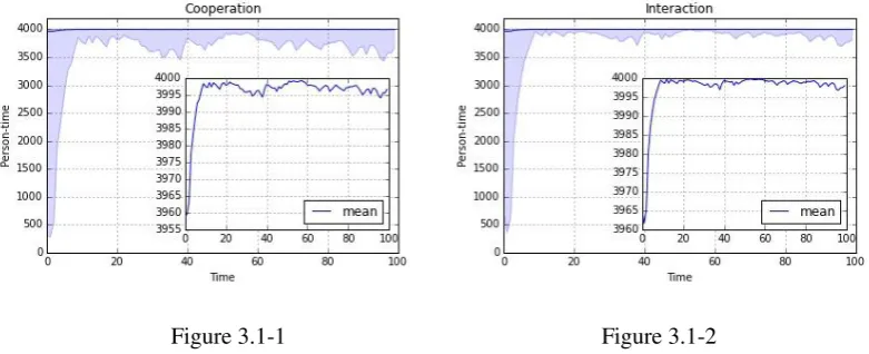
[image:21.595.98.489.307.466.2]The results of base-line simulation are shown in Figure 3.1-1 and Figure 3.1-2. From Figure 3.1-1 and Figure 3.1-2, two variables of interest (namely, person-time of interaction and person-time of cooperation, respectively) undergo a process of approaching to the largest possible value and the distribution of these two variables of interest are largely skew to the left especially in the first 10 time periods.
Figure 3.1-1 Figure 3.1-2
Figure 3.1-1 and Figure 3.1-2 Base-line simulation. Figure 3.1-1 Evolution of person-time of interaction (minimum, mean and maximum). Figure 3.1-2 Evolution of person-time of cooperation (minimum, mean and maximum). Both run 100 times. The blue lines in both big figure and the small figure are the mean values of 100 simulation runs. The light blue shadow in the big figure is the area between minimum and maximum values of the 100 simulation runs.
3.2 Number of immediate neighbors
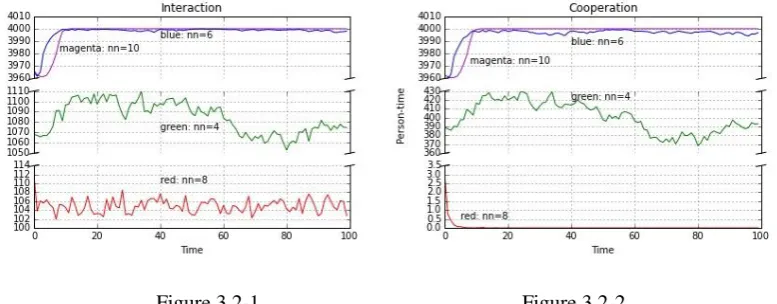
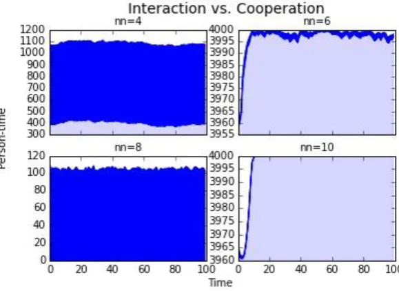
Four different values of number of neighbors, namely nn=4, 6, 8 and 10, with the other parameters having the same value with those in the base-line simulation. The simulation results are shown from Figure 3.2-1 to Figure 3.2-3. From Figure 3.2-1 and Figure 3.2-2, number of immediate neighbors does not exhibit monotonous influence on the two variables of interest: when nn=6 and 10, the two variables of interest situate at high level and rapidly approach to the largest possible values; when nn=4, at lower middle level; when nn=8, at very low level. Additionally, when nn=8, cooperation collapses.
·Impacts on trust
1 𝑃𝑒𝑟𝑠𝑜𝑛𝑇𝑖𝑚𝑒
21
Each agent is a representative of a mixed strategy. On the condition that agents‟ trustworthiness (probability to cooperate) is invariant within a time period, given a particular actual interaction partner, the probabilities of increasing and decreasing personal trust are therewith determined. When nn is relatively small, the probability to meet the same neighbor is relatively high, ceteris paribus. The more times an agent meets the same neighbor, the less probability that he encounters diverse mixed strategies, and the stronger the impact of a particular neighbor‟s trustworthiness on his trust-updating, and the more certain his two trust-updating directions. Thus, encountering the same neighbor reinforces trust-updating directions: the more trustworthy a neighbor, the more opportunities an agent increases trust; the less trustworthy a neighbor, the more chances an agent decreases trust. This influence of number of neighbors on trust therefore is a double-edged sword similar to putting all eggs into one basket. More neighbors offer possibility of dispersing risk of being locked in local environment of trustworthiness constructed by neighbors.
·Impacts on trustworthiness
More neighbors result in less actual interactions with each neighbor and, hence, fewer samples of evaluating the cooperation rate of each neighbor within a time period. This, however, tends to cause polarized evaluation of neighbors, and the “first impression” becomes very important. For example, if an agent carries on one actual interaction with a neighbor, the neighbor‟s cooperation rate can only be 0 or 1. On contrast, if an agent conducts four times of actual interactions with a neighbor, the neighbor‟s cooperation rate can be five values, namely 0, 1/4, 2/4, 3/4 and 1. For example, assume an agent ai‟s trustworthiness is 1/4 and the trustworthiness of his neighbor aj
who receives the most potential interaction requests is 3/4. In the former situation, aj interacts
once in total in a time period and cooperates. aj‟s evaluated cooperation rate will be 1 and ai will
update his trustworthiness to 1. In the latter situation, aj interacts four times and cooperates three
times. aj‟s evaluated cooperation rate will be 3/4 and ai will update his trustworthiness to 3/4. For
another example, assume an agent ai‟s trustworthiness is 1/4 and the trustworthiness of his
neighbor aj who receives the most potential interaction requests is 2/4. In the former situation, aj
interacts once and defects. aj‟s evaluated cooperation rate will be 0 and ai will not update his
trustworthiness and stick to 1/4. In the latter situation, aj interacts four times and cooperates twice.
aj‟s evaluated cooperation rate will be 2/4 and ai will update his trustworthiness to 2/4. This may
[image:22.595.102.491.593.745.2]to some extent explain why the behaviors of the two variables of interest when nn=8 and nn=10 are quite different.
22
Figure 3.2-1 and Figure 3.2-2 Comparison of different values of number of immediate neighbors. Figure 3.2-1 Evolution of mean person-time of interaction. Figure 3.2-2 Evolution of mean person-time of cooperation. Both run 100 times.
Figure 3.2-31 Comparison of different values of number of immediate neighbors. Difference between mean person-time of interaction and cooperation. Run 100 times.
3.3 Degree of embeddedness in social network
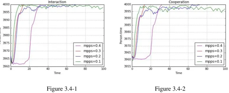
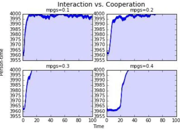
Four different values are compared for degree of embeddedness in social network, namely se=0.6, 0.7, 0.8 and 0.9 with the other six parameters having the same value with those in the base-line simulation. The simulation results are exhibited from Figure 3.3-1 to Figure 3.3-3. From Figure 3.3-1 and Figure 3.3-2, when se=0.8 and 0.9, two variables of interest situate at high level and approach to largest possible value within 20 time periods. On contrast, when se=0.6 and 0,7, the two variables of interest locate very low and mean person-time of cooperation even touches zero. In Figure 3.3-3, when se=0.8 and 0.9, the difference between mean person-time of interaction and that of cooperation is very small; however, when se=0.6 and 0.7, the gap is relatively large. What is more, the gap between person-time of interaction and cooperation exists all the time for all the four candidate values, and the difference is relatively stable.
The principle behind somehow shares the same vein with the impact of number of immediate neighbors on the two variables of interest. When degree of embeddedness in social network is higher, interactions more likely happen within neighborhood, ceteris paribus. Thus, when degree of embeddedness in social network is higher, on one hand, an agent‟s trust-updating relates stronger to his fixed neighbors‟ trustworthiness; on the other hand, an agent has more samples of their neighbors, and more values of cooperation rate and more chances for him to update trustworthiness, which avoid being locked in low trustworthiness trap. Learnt trustworthiness, then, is reflected on interactions. As aforementioned, degree of social embeddedness is an indicator of
1 The relatively dark blue shadow is the difference between mean person-time of interaction and that of
23
social mobility in this paper. Thus, as social mobility accelerates, both trust and trustworthiness may collapse.
[image:24.595.93.489.238.399.2] [image:24.595.138.434.467.677.2]As to the relatively stable gap between mean person-time of interaction and that of cooperation, it may be attributed to: 1) Information acquisition capability. Assume an agent whose current trust is low. If his information acquisition capability via observing (both neighbors and non-neighbors) is at the same time low, then he has fewer chances to increase trust and will always not participate in actual interactions. 2) Unilateral link weights updating. An agent‟s most defective neighbor has less likelihood to be chosen as a potential interaction partner if other neighbors are more cooperative.
Figure 3.3-1 Figure 3.3-2
Figure 3.3-1 and Figure 3.3-2 Comparison different values of degree of embeddedness in social network. Figure 3.3-1 Evolution of mean person-time of interaction. Figure 3.3-2 Evolution of mean person-time of cooperation. Both run 100 times.
Figure3.3-3 Comparison of different values of degree of embeddednss in social network. Difference between mean person-time of interaction and cooperation. Run 100 times.