Computing Lexical Chains with Graph Clustering

Computing Lexical Chains with Graph Clustering

Olena Medelyan

Computer Science Department

The University of Waikato

New Zealand

olena@cs.waikato.ac.nz

Abstract

This paper describes a new method for computing lexical chains. These are sequences of semantically related words that reflect a text’s cohesive structure. In contrast to previous methods, we are able to select chains based on their cohesive strength. This is achieved by analyzing the connectivity in graphs representing the lexical chains. We show that the generated chains significantly improve performance of automatic text summarization and keyphrase indexing.

1

Introduction

Text understanding tasks such as topic detection, automatic summarization, discourse analysis and question answering require deep understanding of the text’s meaning. The first step in determining this meaning is the analysis of the text’s concepts and their inter-relations. Lexical chains provide a framework for such an analysis. They combine semantically related words across sentences into meaningful sequences that reflect the cohesive structure of the text.

Lexical chains, introduced by Morris and Hirst (1991), have been studied extensively in the last decade, since large lexical databases are available in digital form. Most approaches use WordNet or Roget’s thesaurus for computing the chains and apply the results for text summarization.

We present a new approach for computing lexical chains by treating them as graphs, where

nodes are document terms and edges reflect semantic relations between them. In contrast to previous methods, we analyze the cohesive strength within a chain by computing the diameter of the chain graph. Weakly cohesive chains with a high graph diameter are decomposed by a graph clustering algorithm into several highly cohesive chains. We use WordNet and alternatively a domain-specific thesaurus for obtaining semantic relations between the terms.

We first give an overview of existing methods for computing lexical chains and related areas. Then we discuss the motivation behind the new approach and describe the algorithm in detail. Our evaluation demonstrates the advantages of using extracted lexical chains for the task of automatic text summarization and keyphrase indexing, compared to a simple baseline approach. The results are compared to annotations produced by a group of humans.

2

Related Work

Morris and Hirst (1991) provide the theoretical background behind lexical chains and demonstrate how they can be constructed manually from Roget’s thesaurus. The algorithm was re-implemented as soon as digital WordNet and Roget’s became available (Barzilay and Elhadad, 1997) and its complexity was improved (Silber and McCoy, 2002; Galley and McKeown, 2003). All these algorithms perform explicit word sense disambiguation while computing the chains. For each word in a document the algorithm chooses only one sense, the one that relates to members of existing lexical chains. Reeve et al. (2006)

compute lexical chains with a medical thesaurus and suggest an implicit disambiguation: once the chains are computed, weak ones containing irrelevant senses are eliminated. We also follow this approach.

One of the principles of building lexical chains is that each term must belong to exactly one chain. If several chains are possible, Morris and Hirst (1991) choose the chain to whose overall score the term contributes the most. This score is a sum over weights of semantic relations between chain members. This approach produces different lexical chains depending on the order of words in the document. This is not justified, as the same content can be expressed with different sequences of statements. We propose an alternative order independent approach, where a graph clustering algorithm calculates the chain to which a term should belong.

3

Lexical Chains

The following notation is used throughout the paper. A lexical chain is a graph G = (V,E) with nodes viV being terms and edges (vi,vj,wij)E representing semantic relations between them, where wij is a weight expressing the strength of the relation.1 A set of terms and semantic relations building a graph is a valid lexical chain if the graph is connected, i.e. there are no unconnected nodes and no isolated groups of nodes.

The graph distance d(vi, vj) between two nodes

vi and vj is the minimum length of the path connecting them. And the graph diameter is the “longest shortest distance” between any two nodes in a graph, defined as:

(1) m max_v,v d(v_i,v_j)

j i

 .

1

The initial experiments presented in this paper use an

unweighted graph with wi,j = 1 for any semantic relation.

Because semantic relations are either bi-directional or inverse, we treat lexical chains as

undirected graphs.

3.1 The Cohesive Strength

Lexical cohesion is the property of lexical entities to “stick together” and function as a whole (Morris and Hirst, 1991). How strongly the elements of a lexical chain “stick together,” that is the cohesive strength of the chain, has been defined as the sum of semantic relations between every pair of chain members (e.g. Morris and Hirst, 1991; Silber and McCoy, 2002). This number increases with the length of a chain, but longer lexical chains are not necessarily more cohesive than shorter ones.

Instead, we define the cohesive strength as the diameter of the chain graph. Depending on their diameter we propose to group lexical chains as follows:

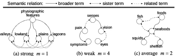
1. Strongly cohesive lexical chains (Fig. 1a) build fully connected graphs where each term is related to all other chain members andm = 1.

2. Weakly cohesive lexical chains (Fig. 1b) connect terms without cycles and with a diameter

m = |V|  1.

3. Moderately cohesive lexical chains (Fig. 1c) are in-between the above cases with m[1, |V|1].

To detect individual topics in texts it is more useful to extract strong lexical chains. For example, Figure 1a describes “physiographic features” and 1c refers to “seafood,” while it is difficult to summarize the weak chain 1b with a single term. The goal is to compute lexical chains with the highest possible cohesion. Thus, the algorithm must have a way to control the selection.

physiographic features

valleys lowland plains lagoons

(a) strong m = 1

symptoms eyes

vision senses

pain

(b) weak m = 4

shelfish seafoods

squids

foods fish

(c) average m = 2

Semantic relation: broader term sister term related term

physiographic features

valleys lowland plains lagoons

(a) strong m = 1

symptoms eyes

vision senses

pain

(b) weak m = 4

shelfish seafoods

squids

foods fish

(c) average m = 2

Semantic relation: broader term sister term related term

3.2 Computing Lexical Chains

The algorithm consists of two stages. First, we compute lexical chains in a text with only one condition: to be included into a chain a term needs to be related to at least one of its members. Then, we apply graph clustering on the resulting weak chains to determine their strong subchains.

I. Determining all chains.First, the documents’ n-grams are mapped onto terms in the thesaurus. To improve conflation we ignore stopwords and sort the remaining stemmed words alphabetically. Second, for each thesaurus term t that was found in the document we search for an appropriate lexical chain. We iterate over the list L containing previously created chains and check whether term t

is related to any of the members of each chain. The following cases are possible:

1. No lexical chains were found.

A new lexical chain with the term tas a single element is created and included inL. 2. One lexical chain was found.

This chain is updated with the term t. 3. Two or more lexical chains were found.

We merge these chains into a single new chain, and remove the old chains from L.

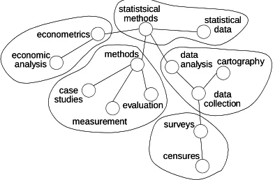
II. Clustering within the weak chains.

Algorithms for graph clustering divide sparsely connected graphs into dense subgraphs with a similar diameter. We consider each lexical chain in

L with diameter m3as a weak chain and apply graph clustering to identify highly cohesive subchains within this chain. The list L is updated with the newly generated chains and the original chain is removed.

A popular graph clustering algorithm, Markov Clustering (MCL) is based on the idea that “a random walk that visits a dense cluster will likely not leave the cluster until many of its vertices have been visited” (van Dongen, 2000). MCL is implemented as a sequence of iterative operations on a matrix representing the graph. We use ChineseWhispers (Biemann, 2006), a special case of MCL that performs the iteration in a more aggressive way, with an optimized linear complexity with the number of graph edges.

Figure 2 demonstrates how an original weakly cohesive lexical chain has been divided by ChineseWhispers into five strong chains.

4

Lexical Chains for Text Summarization

Lexical chains are usually evaluated in terms of their performance on the automatic text summarization task, where the most significant sentences are extracted from a document into a summary of a predefined length. The idea is to use the cohesive information about sentence members stored in lexical chains. We first describe the summarization approach and then compare results to manually created summaries.

4.1 Identifying the Main Sentences

The algorithm takes one document at a time and computes its lexical chains as described in Section 3.2, using the lexical database WordNet. First, we consider all semantic senses of each document term. However, after weighting the chains we eliminate senses appearing in low scored chains.

Doran et al. (2004) state that changes in weighting schemes have little effect on summaries. We have observed significant differences between reported functions on our data and achieved best results with the formula produced by Barzilay and Elhadad (1997):

(2)







 



LC t LC

t

t freq t

freq LC LC

Score ) ()

) ( | | 1 ( ) (

Here, |LC| is the length of the chain and freq(t) is the frequency of the term t in the document. All lexical chains with score lower than a threshold contain irrelevant word senses and are eliminated.

Next we identify the main sentences for the final summary of the document. Different heuristics have been proposed for sentence extraction based on the information in lexical chains. For each top scored chain, Barzilay and Elhadad (1997) extract

econometrics

statistsical methods

economic analysis

case studies

methods

measurement evaluation

statistical data

data

analysis cartography

data collection

surveys

censures econometrics

statistsical methods

economic analysis

case studies

methods

measurement evaluation

statistical data

data

analysis cartography

data collection

surveys

censures

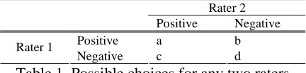
Rater 2

Positive Negative

Positive a b

Rater 1

Negative c d

Table 1. Possible choices for any two raters

that sentence which contains the first appearance of a chain member. Doran et al. (2004) sum up the weights all words in the sentence, which correspond to the chain weights in which these words occur. We choose the latter heuristic because it significantly outperforms the former method in our experiments.

The highest scoring sentences from the document, presented in their original order, form the automatically generated summary. How many sentences are extracted depends on the requested summary length, which is defined as the percentage of the document length.

4.2 Experimental Settings

For evaluation we used a subset of a manually annotated corpus specifically created to evaluate text summarization systems (Hasler et al. 2003). We concentrate only on documents with at least two manually produced summaries: 11 science and 29 newswire articles with two summaries each, and 7 articles additionally annotated by a third person. This data allows us to compare the consistency of the system with humans to their consistency with each other.

The results are evaluated with the Kappa statistic , defined for Table 1 as follows:

(3)

) )( ( ) 9 )( (

) ( 2

b a d b c

c a

bc ab

    

 



It takes into account the probability of chance agreement and is widely used to measure inter-rater agreement (Hripcsak and Rothshild, 2005). The ideal automatic summarization algorithm should have as high agreement with human subjects as they have with each other.

We also use a baseline approach (BL) to estimate the advantage of using the proposed lexical chaining algorithm (LCA). It extracts text summaries in exactly the manner described in Section 4.1, with the exception of the lexical chaining stage. Thus, when weighting sentences, the frequencies of all WordNet mappings are taken into account without the implicit word sense disambiguation provided by lexical chains.

Humans BL LCA

S1 0.19 0.20

29 newswire

articles S2 0.32 0.20 0.24

S1 0.08 0.13

11 science

articles S2 0.34 0.13 0.22

Table 2. Kappa agreement on 40 summaries

vs. human

2,3 and 1 vs. BL vs. LCA

human 1 0,41 0,30 0,30

human 2 0,38 0,22 0,24

human 3 0,28 0,17 0,24

average 0,36 0,23 0,26

Table 3. Kappa agreement on 7 newswire articles

4.3 Results

Table 2 compares the agreement among the human annotators and their agreement with the baseline approach BL and the lexical chain algorithm LCA. The agreement between humans is low, which confirms that sentence extraction is a highly subjective task. The lexical chain approach LCA significantly outperforms the baseline BL, particularly on the science articles.

While the average agreement of the LCA with humans is still low, the picture changes when we look at the agreement on individual documents. Human agreement varies a lot (stdev= 0.24), while results produced by LCA are more consistent (stdev= 0.18). In fact, for over 50% of documents LCA has greater or the same agreement with one or both human annotators than they with each other. The overall superior performance of humans is due to exceptionally high agreement on a few documents, whereas on another couple of documents LCA failed to produce a consistent summary with both subjects. This finding is similar to the one mentioned by Silber and McCoy (2002).

Table 3 shows the agreement values for 7 newswire articles that were summarized by three human annotators. Again, LCA clearly outperforms the baseline BL. Interestingly, both systems have a greater agreement with the first subject than the first and the third human subjects with each other.

5

Lexical Chains for Keyphrase Indexing

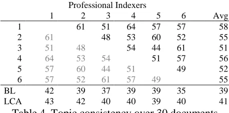
Professional Indexers

1 2 3 4 5 6 Avg

1 61 51 64 57 57 58

2 61 48 53 60 52 55

3 51 48 54 44 61 51

4 64 53 54 51 57 56

5 57 60 44 51 49 52

6 57 52 61 57 49 55

BL 42 39 37 39 39 35 39

LCA 43 42 40 40 39 40 41

Table 4. Topic consistency over 30 documents

document terms individually. Lexical chains enable

topical indexing, where first highly cohesive terms are organized into larger topics and then the main topics are selected. Properties of chain members help to identify terms that represent each keyphrases. To compute lexical chains and assign keyphrases this time we use a domain-specific thesaurus instead of WordNet.

5.1 Finding Keyphrases in Lexical Chains

The ranking of lexical chains is essential for determining the main topics of a document. Unlike in summarization, it should capture the specificity of the individual chains. Also, for some topics, e.g. proper nouns, the number of terms to express it can be limited; therefore we average frequencies over all chain members. Our measure of chain specificity combines TFIDFs and term length,2 which boosts chains containing specific terms that are particularly frequent in a given document:

(4)

LC

t length t

TFIDF LC

Score t





 

) ( )

( )

(

We assume that the top ranked weighted lexical chains represent the main topics in a document. To determine the keyphrases, for each lexical chain we need to choose a term that describes this chain in the best way, just as “seafood” is the best descriptor for the chain in Figure 1c.

Each member of the chain t is scored as follows:

(5) Score(t)TFIDF(t)ND(t)length(t)

where ND(t) is the node degree, or the number of edges connecting term t to other chain members. The top scored term is chosen as a keyphrase.

2 _{Term length, measured in words, gives an indirect but}

simple measure of its specificity. E.g., “tropical rain forests” is more specific than “forests”.

Professional indexers tend to choose more than one term for a document’s most prominent topics. Thus, we extract the top two keyphrases from the top two lexical chains with |LC|  3. If the second keyphrase is a broader or a narrower term of the first one, this rule does not apply.

5.2 Evaluation of the Extracted Keyphrases

This approach is evaluated on 30 documents indexed each by 6 professional indexers from the UN’s Food and Agriculture Organization. The keyphrases are driven from the agricultural thesaurus Agrovoc3with around 40,000 terms and 30,000 semantic relations between them.

The effectiveness of the lexical chains is shown in comparison to a baseline approach, which given a document simply defines keyphrases as Agrovoc terms with top TFIDF values.

Indexing consistency is computed with the F-Measure F, which can be expressed in terms of Table 1 (Section 4.1) as following:4

(6)

c b a

a F

  

2 2

The overlap between two keyphrase sets a is usually computed by exact matching of keyphrases. However, discrepancies between professional human indexers show that there are no “correct” keyphrases. Capturing main topics rather than exact term choices is more important. Lexical chains provide a way of measuring this so called

topical consistency. Given a set of lexical chains extracted from a document, we first compute chains that are covered in its keyphrase set and then compute consistency in the usual manner.

5.3 Results

Table 4 shows topical consistency between each pair of professional human indexers, as well as between the indexers and the two automatic approaches, baseline BL and the lexical chain algorithm LCA, averaged over 30 documents.

The overall consistency between the human indexers is 55%. The baseline BL is 16 percentage points less consistent with the 6 indexers, while

3_{http://www.fao.org/agrovoc/}

4_{When vocabulary is large, the consistency is the same,}

LCA is 1 to 5 percentage points more consistent with each indexer than the baseline.

6

Discussion

Professional human indexers first perform conceptual analysis of a document and then translate the discovered topics into keyphrases. We show how these two indexing steps are realized with lexical chain approach that first builds an intermediate semantic representation of a document and then translates chains into keyphrases. Conceptual analysis with lexical chains in text summarization helps to identify irrelevant word senses.

The initial results show that lexical chains perform better than baseline approaches in both experiments. In automatic summarization, lexical chains produce summaries that in most cases have higher consistency with human annotators than they with each other, even using a simplified weighting technique. Integrating lexical chaining into existing keyphrase indexing systems is a promising step towards their improvement.

The lexical chaining does not require any resources other than a controlled vocabulary. We have shown that it performs well with a general lexical database and with a domain-specific thesaurus. We use the Semantic Knowledge Organization Standard5which allows easy inter-changeability of thesauri. Thus, this approach is domain and language independent.

7

Conclusions

We have shown a new method for computing lexical chains based on graph clustering. While previous chaining algorithms did not analyze the lexical cohesion within each chain, we force our algorithm to produce highly cohesive lexical chains based on the minimum diameter of the chain graph. The required cohesion can be controlled by increasing the diameter value and adjusting parameters of the graph clustering algorithm.

Experiments on text summarization and key-phrase indexing show that the lexical chains approach produces good results. It combines symbolic analysis with statistical features and

5_{http://www.w3.org/2004/02/skos/}

outperforms a purely statistical baseline. The future work will be to further improve the lexical chaining technique and integrate it into a more complex topical indexing system.

8

Acknowledgements

I would like to thank my PhD supervisors Ian H. Witten and Eibe Frank, as well as Gordon Paynter and Michael Poprat and the anonymous reviewers of this paper for their valuable comments. This work is supported by a Google Scholarship.

References

Chris Biemann 2006. Chinese Whispers—an Efficient Graph Clustering Algorithm and its Application to

Natural Language Processing Problems. In Proc of

the HLT-NAACL-06 Workshop on Textgraphs, pp. 73-80.

Regina Barzilay and Michael Elhadad. 1997. Using

Lexical Chains for Text Summarization, In Proc of

the ACL Intelligent Scalable Text Summarization Workshop, pp. 10-17.

Stijn M. van Dongen. 2000. Graph Clustering by Flow

Simulation. PhD thesis, University of Utrecht.

William P. Doran, Nicola Stokes, Joe Carthy and John Dunnion. 2004. Assessing the Impact of Lexical

Chain Scoring Methods on Summarization. In Proc of

CICLING’04, pp. 627-635.

Laura Hasler, Constantin Orasan and Ruslan Mitkov. 2003. Building Better Corpora for Summarization. In

Proc of Corpus Linguistics CL’03, pp. 309-319.

George Hripcsak and Adam S. Rothschild. 2005. Agreement, the F-Measure, and Reliability in IR.

JAMIA, (12), pp. 296-298.

Jane Morris and Graeme Hirst. 1991. Lexical Cohesion Computed by Thesaural Relations as an Indicator of

the Structure of Text. Computational Linguistics,

17(1), pp. 21-48.

Lawrence H. Reeve, Hyoil Han and Ari D. Brooks. 2006. BioChain: Using Lexical Chaining for

Biomedical Text Summarization. In Proc of the ACM

Symposium on Applied Computing, pp. 180-184.

Gregory Silber and Kathleen McCoy, 2002. Efficiently Computed Lexical Chains as an Intermediate Representation for Automatic Text Summarization.