Munich Personal RePEc Archive
Historical trades, skills and
agglomeration economies
Ehrl, Philipp and Monteiro Monasterio, Leonardo
Universidade Católica de Brasília, IPEA
7 April 2016
Online at
https://mpra.ub.uni-muenchen.de/69829/
Historical trades, skills and agglomeration
economies
⋆Philipp Ehrl‡
Universidade Católica de Brasília
Leonardo Monasterio
Universidade Católica de Brasília, IPEA, UCLA
April 7, 2016
Abstract
We exploit differences in the spatial distribution of industrial and liberal occu-pations in the years 1872 and 1920 to instrument for today’s concentration of inter-personal and analytical skills in Brazil. The data suggest that the local supply of knowledge and manufacturing provided by these historical trades favored a growth path that has shaped the occupational structure until the present day, whereby the existence of a large local consumer market was a necessary condition for this devel-opment. By means of these instruments, we present causal evidence that the regional concentration of interpersonal and analytical skills generates positive wage externali-ties. Particularly university graduates and workers without formal education benefit most from these agglomeration economies.
Keywords: agglomeration economies, skills, long-run industrial development, Brazil JEL Classification: R12, J31, C26, N16
⋆
We thank Daniel da Mata and seminar participants at the UCLA, NARSC, CIDE, IPEA in Brasília and the UCB for the discussions and valuable comments. Ehrl gratefully acknowledges financial support from CAPES.
‡corresponding author: Universidade Católica de Brasília, Post-Graduate Program in Economics, SGAN
1
Introduction
"(2) The scale of an industrial plant depends on the demand for its products [...] (7) Since it takes machines to produce machines, and these are themselves the product of many different factories and workshops, machinery is produced efficiently only in a place where factories and workshops are close enough to-gether to help each other work in unison, i.e. in large towns".
— (von Thünen 1826/1966: 287-90),The Isolated State
Plants benefit from locating close to each other in large towns for two reasons listed in the initial quote: the positive interaction between economies of scale (supply) and the consumer market (demand); and the benefits due to the cooperation and exchange between different producers. In consonance, Marshall (1890) used the famous expression "mysteries of the trades" to paraphrase how people benefit from a concentration of workers with the "same skilled trade" through positive externalities. Arrow (1962) provides the related insight that physical production itself is required for "learning by doing". We aim to test the empirical content of these arguments, i.e., we evaluate the linkages among the concentration of knowledge and production, agglomeration economies and long-run growth.
The present paper makes two main contributions to the literature. (1) As far as we know, we are the first to present causal evidence that the spatial concentration of interactive and analytic skills generates positive externalities for workers’ wages.1 A general problem with
the identification of agglomeration economies is their endogeneity due to reverse causality and the sorting of workers to high-wage regions according to unobservable abilities (Combes et al.2008). (2) To tackle this endogeneity problem and the measurement error in the skill variables, we exploit differences in the spatial distribution of industrial and liberal occu-pations from the Brazilian Censuses in 1872 and 1920 to construct instrumental variables. The identification assumption rests on the argument that the regional concentration of these professions in the past stimulated sustainable long-run economic growth and thus resulted in a high conglomeration of analytic and interactive skills today.
A preliminary analysis of the Brazilian data reveals that interactive and analytic skills are heavily concentrated in densely populated regions. The same applies to managers, scientists and skilled technicians, which correspond to the type of occupations with the highest wages/skills. The corollary is that manual skills can primarily be found in rural regions. Maciente (2013) also studies the distribution of skills in Brazil with different skill definitions but comes to the same basic conclusions. Similar observations are reported for the US by Bacolod et al. (2009b), Florida et al. (2012) and as well as for Sweden by Anderssonet al.(2014). Moreover, Bacolodet al.(2009a) observe that returns to cognitive and interactive skills grow with the size of the region. These results are suggestive that in the modern economy, the agglomeration economies mainly arise from the interpersonal exchange of ideas and knowledge spillovers. Thus far, these insights have been merely
1
based on simple correlations so to make progress instrumental variables are introduced here. We are convinced that the chosen instruments are valid for the following reasons.
Industrialist is one of the professions distinguished in the Census of 1872, the era of the very beginning of the industrialization in Brazil. Industrialists were the owners of factories and their factories provided jobs and generated capital which could be reinvested to expand and continually modernize the production. On the other hand, liberal professions (such as lawyers, judges, professors and teachers) generated knowledge – a scarce and highly valuable asset at that time – and contributed to the functioning of the fragile institutions. As argued above, the local accumulation of knowledge and physical production were key to productivity increases and the sustained economic growth that eventually led to the local development of ever more modern and dynamic industries. A region with predominantly agricultural workers, domestic servants and individuals without a profession, in contrast, hindered the development of the local economy and preserved the ancient structures. An econometric test of these theories over a long period is, to the best of our knowledge, absent thus far. Moreover, we observe that positive progress was much more likely if the region was a large agglomeration already. This suggests that the interaction between supply (provided by the industrialists) and consumer demand created a virtuous cycle for the local economy. Thus, market potential, circular linkages, and history do play a crucial role in the development of agglomerations, as predicted by the theories of the New Economic Geography (Fujitaet al.2001).
Since Ciccone and Hall (1996), regional economists have used historical variables to in-strument for the population size or density of regions, exploiting the persistence of large settlements per se. Alternatively, Rosenthal and Strange (2008) and Combeset al.(2010) use characteristics of the subsoil since these factors influenced agricultural yields which represented a major reason for the establishment of early settlements. The difference with our paper is that size and density proxy for various observably equivalent agglomeration economies. However, the skill concentration exposes a specific externality. Robustness checks show that our instruments are neither driven by the historic size of regions, nor does additionally controlling (and instrumenting) for population size alter our findings.
A related approach in Acemoglu et al. (2001), is based on variation in settler mortality rates in the 16th
century as an instrument for the differing quality of institutions in or-der to explain countries’ diverging development paths. Other papers that focus on the exploitation of natural resources, forced labor and institutions are those of Nunn (2008), Dell (2010) and Naritomiet al. (2012). In our approach industrial structures in the past provide a link to the current concentration of occupations and skills in regions within a single country. First nature advantages like proximity to the sea and railroads turn out to have a slight impact on the current wage distribution without, however, undermining the IVs’ relevance.
personal characteristics, sectoral affiliation, regional differences and permanent first nature advantages. Specifically, we find that an increase of one standard deviation in the local concentration of skills raises the average wage level in a region by about 10%. A large divergence between OLS and IV estimates indicates that endogeneity and measurement error in skills are substantial. Note, however, that none of our findings crucially hinges on the utilization of skill variables. We observe comparable wage effects from the concentration of managers, scientists and skilled technicians, i.e., those workers that use analytic and interpersonal skills most intensively. Since these skills are especially concentrated in large, urban regions, our paper also contributes to the explanation of the urban wage premium, cf. Glaeser and Maré (2001).
The paper most closely related to ours is Michaels et al. (2013). Those authors report for the US that in 1880 it was mainly manual/physical skills that were concentrated in urban areas, while nowadays, mostly interactive skills are located there. They provide a general equilibrium model with multiple regions, sectors, occupations and task/skills that explains this structural transformation of the economy. In essence, they conclude that the nature of agglomeration economies has changed over time. Due to falling transport and task trade costs, the benefits of concentrating physical production have diminished, while the concentration of interactive skills in densely populated regions has become more attractive. This argument is perfectly consistent with our findings. Yet not all densely populated regions exhibit a high concentration of interactive skills. Our paper adds to the picture that the transition of regions to the current equilibrium did not occur arbitrarily but was largely favored by the regions’ sectoral supply and demand capacity in the past.2
Moreover, we link the distribution of historical and current occupations to information about individuals, including their wages.
One of the few papers that also applies econometric methods to analyze the long-run economic development since 1872 in Brazil is Reis (2014). He also acknowledges the im-portance of both geographic factors and institutions (such as slavery) in explaining the persistent regional income inequality in Brazil. The paper documents the slow conversion of income per capita and labor productivity, i.e., the persistence of regional inequality patterns.
Finally, our approach is also related to papers on the dynamic aspect of agglomeration externalities and long-run economic development. Glaeser et al. (1992) examine city-industries over a period of 22 years to test whether industrial specialization, competition of diversity is more favorable for employment growth. The difference between our study and theirs is that they focus on the development of single localized industries and on em-ployment growth directly, whereas we investigate long-term transitions from the industrial revolution up to the present day. Hendersonet al.(1995: 1068) also acknowledge that dy-namic externalities "lead to a buildup of local trade secrets". Again, the analyzed period in their study does not exceed 30 years.
2
The remainder of the paper is organized as follows. Section 2 explains our estimation strategy. Section 3 reviews the historical background in Brazil and section 4 describes the utilized data. Section 5 contains the results and further robustness checks. Section 6 concludes the paper.
2
Estimating the agglomeration economies of skills
To identify the agglomeration economies of skills we start with two linear wage regres-sions. The two models incorporate skills and agglomeration economies in different ways. Both models include the log population size (𝑠𝑖𝑧𝑒ik) of region 𝑘where individual 𝑖 works
in order to account for the multitude of observably equivalent agglomeration advantages (Rosenthal and Strange 2004). Beyond that, we exploit skill measures that we derive from the occupation of each individual worker in our sample. The precise definition of our skill variable is contained in section 4.3.
In the first approach, we capture the effect of skills through the average value of the skill variable in region𝑘. The estimation equation thus reads
𝑤ik =𝛽1𝑠𝑘𝑖𝑙𝑙ik+𝛽2𝑠𝑖𝑧𝑒ik+𝑐𝑜𝑛𝑡𝑟𝑜𝑙𝑠i+𝛿io+𝜖ik (1)
where 𝑤ik is the log hourly wage of individual 𝑖 and 𝑐𝑜𝑛𝑡𝑟𝑜𝑙𝑠i represent workers’
socio-economic characteristics provided in the census for 2010 (cf. section 4.1) namely: age and age2, education, race, marital status, occupational position, gender, having a physical difficulty, being illiterate or a foreigner. The term𝑐𝑜𝑛𝑡𝑟𝑜𝑙𝑠i also includes some fixed effects
to control for general wage differences between sectors and Federal States. Because the two variables of interest (𝑠𝑘𝑖𝑙𝑙ik and 𝑠𝑖𝑧𝑒ik) only have variation at the regional level, clustered
standard errors are required (Moulton 1986). As in all of the following estimations, we use the sample weights provided by the Census.
Despite these individual controls, the average wage in a region may simply be higher because many white-collar workers are located there. This circumstance would go hand in hand with a high average skill score. Yet our aim is to distinguish the pure externality of the skill concentration from the average wage level which comes along mechanically with the occupational composition. Using occupation fixed effects𝛿io (at the 2-digit level),
we eliminate both the effect of individual skills as well as all other differences between professions that have an impact on wages, such as unobserved skills that are common within a peer group.
In the second model, we estimate how the hedonic price of skills varies with the local pop-ulation size following Bacolodet al. (2009a). Thereby, our data and implied externalities can be directly compared with a related study from the US. In contrast to eq. (1), the skill value of individual𝑖’s occupation enters the equation directly, and only the coefficient of
the interaction term𝛾3 informs about whether the hedonic price of the 𝑠𝑘𝑖𝑙𝑙differs among regions.
The term𝑐𝑜𝑛𝑡𝑟𝑜𝑙𝑠i represent the same variables as in eq. (1) above. However, we cannot
include occupation fixed effects because the variable𝑠𝑘𝑖𝑙𝑙io only has variation at the
occu-pation level. Since𝑠𝑖𝑧𝑒ik is another aggregated variable, standard errors are clustered at
the region-occupation level here.
Obviously, the interpretations of the coefficients of interest (𝛽1 and𝛾3) are different in the two specifications. For ease of interpretation all independent variables (except for dummy variables) are centered on their weighted sample mean. Thus, in the second model, the sum
𝛾1+𝛾3indicates the marginal wage effect that occurs if an individual𝑖who lives in a region of medium size is employed in an occupation that demands slightly more of the specific
𝑠𝑘𝑖𝑙𝑙 category than the average worker in the economy is performing. The interaction
effect 𝛾3 also shows if the hedonic price of the skill varies according to the size of the region. A positive coefficient indicates that performing a specific type of skill becomes more productive in the presence of any kind of other workers. In contrast,𝛽1 >0 in the first model indicates that every worker, independent of his/her occupation, benefits from a higher concentration of a specific skill. In fact, eq. (1) measures a specific agglomeration advantage while eq. (2) expresses the general advantage of size for a specific activity. For this reason and because it also the path of least econometric resistance we prefer to work with the concentration of skills at the regional level as our main variable of interest. The specification with the interaction term between two endogenous variables is especially inappropriate when it comes to instrumenting for these variables, as we discuss below. Therefore, eq. (1) is continually enhanced during the rest the analysis.
Several threats to the identification of agglomeration economies arise in the OLS regres-sions. These can be summarized under the three well-known keywords: measurement error, omitted variables and reverse causality. First, large cities with the highest wages attract the best workers, just like Frank Sinatra said about New York: "if I can make it there, I’ll make it anywhere".3 An immediate consequence is that an influx of high-wage workers
in-creases the average wage in the region, so that ever more high-wage workers are attracted, and so on and and so forth. Another problem with this selection of the best individuals to large regions is that, most likely, not all relevant wage determinants can be captured through education and the remainder observable personal characteristics. Thus wages may vary due to unobservables and as the study of Combeset al.(2008) or Ehrl (2014a) shows, this is especially true in populated regions. The problem in the present case is that work-ers with high wages and high unobserved skills are mainly also those who use analytical and interpersonal skills intensively. For these two reasons, the skill concentration is an endogenous variable and its OLS regression coefficient is generally biased.
In addition, measurement error may be present in each individual skill value. The values in the data are averages at the level of occupations extracted from representative surveys. However, it may be that the intensity of skills differs among regions. As argued above, workers who possess the best observable characteristics may use face-to-face skills more
3
intensively than people who formally have the same profession, but are employed in rural areas. Finally, the fact that a representative survey on skill data is absent in Brazil and we resort to data from the United States, may induce deviations from the true skill values, too. It is well known that due to this attenuation bias the estimated coefficients are closer to zero than their true value. The good news is that all three problems are mitigated at once by the use of instrumental variables.
From historical data from the years 1872 and 1920, we generate four instrumental variables so that it is possible to assess the exogeneity of the instruments with overidentification tests.4 Building on eq. (1), we estimate the following three versions thereof in order to
deepen our understanding of the underlying agglomeration mechanisms
𝑤ik =𝛽1𝑠𝑘𝑖𝑙𝑙ik+𝑐𝑜𝑛𝑡𝑟𝑜𝑙𝑠i+𝛿io (3)
𝑤ik =𝛽1𝑠𝑘𝑖𝑙𝑙ik+𝑐𝑜𝑛𝑡𝑟𝑜𝑙𝑠i+𝛿io
for highly populated regions in 1872/1920
for rural regions in 1872/1920 (4)
𝑤ik =𝛽1𝑠𝑘𝑖𝑙𝑙ik+𝛽2𝑠𝑖𝑧𝑒ik+𝑐𝑜𝑛𝑡𝑟𝑜𝑙𝑠i+𝛿io (5)
where 𝑠𝑘𝑖𝑙𝑙ik and 𝑠𝑖𝑧𝑒ik are instrumented by one or more IVs. Running the regressions
at the individual level is more suitable than at the regional level due to the multitude of worker-specific control variables. As an example, controlling for (mean) education at the regional level is inopportune, since the overall education level may be correlated with the size of the region, which makes education another endogenous variable. Instrument-ing for one more endogenous variable is technically possible but not desirable because it complicates the interpretation of the results. This is why we avoid estimations with an interaction term of two endogenous variables, such as eq. (2). For the same reason, we prefer eq. (3) over eq. (5) where the term𝑠𝑖𝑧𝑒ik partials out other types of agglomeration
economies. The latter variable is indisputably as endogenous as the skill concentration measure. Nevertheless, as a robustness check, we control and additionally instrument for the current population size of regions.
Finally, we split the sample according to the historical size of regions in eq. (4). On the one hand, one can infer whether the agglomeration effects are heterogeneous, in a similar way to an interaction between the skill concentration and the size of the region. At the same time, one avoids the above-mentioned problems related to multiple IVs. On the other hand, we will argue below that the relation between the the historical IVs and the endogenous skill concentrations is significantly stronger if the region had a large population in the past. For this reason, we distinguish regions according to their size in 1872 and 1920, respectively, depending on the year of the instruments in use.
Estimations of eq. (3) to eq. (4) are primarily made with 2SLS. If more than one IV is used, estimation with GMM is more efficient (Baum et al. 2007). Except for eq. (2), standard errors are clustered at the regional level to account for spatial correlations across
4
regions. Other cluster levels and combinations with the occupation-level are certainly possible but as in Rosenthal and Strange (2008: 381) we observe that in comparison to other clustering strategies, the clustering at the most aggregated, i.e., the regional level, is "a conservative approach in the sense that it has the greatest downward impact on the model test statistics". Clustered error terms complicate the calculation of the usual IV test statistics somewhat because most of the tests are based on i.i.d. errors in their original formulation. In the GMM estimations, the exogeneity of the instruments is tested by means of Hansen’s J statistic which allows observations to be correlated within groups. A robustified version of Kleibergen’s K statistic is used according to Finlayet al. (2013). This K statistic indicates whether the estimated coefficient is significantly different from zero assuming that the IV is exogenous. We also apply the widely recognized test for weak instruments by Stock and Yogo (2005) in its cluster-robust version provided by Olea and Pflüger (2013) which, however, is only applicable in the case of one endogenous variable.
3
Historical background
In 1872, Brazil was an undemocratic, rural, sparsely populated, slave-owning society and above all very poor. Its per capita income was only 1.8 times the subsistence level, similar to Malawi or poorer than Rwanda or Somalia today; and 16% of the population were slaves (The Maddison-Project 2010). When compared to other countries, its per capita income was half that observed in Argentina and just over a fifth of England’s. Brazilians’ life expectancy at birth was only 27.4 years and population density was 1.2 inhabitant per square kilometer (lower than contemporary Mongolia) (Mello 1984). In 1872, the great wave of non-Iberian immigration had not yet arrived with full force. Excluding those born in Portugal and Africa, there were only 120,000 foreigners in the country. The big wave of immigrants – many of whom possessed better skills than the average Brazilian – gained pace from the last quarter of the 19th
century onward. By 1920, Brazilian population had reached 30 million, of which 1.6m were foreigners or naturalized (Levy 1974: 79).
In 1872, the majority the almost 10 million inhabitants lived in municipalities close to the sea. The enormous size of the country and the Serra do Mar – a mountain range parallel to the Atlantic coast – have historically imposed high transportation costs on Brazil. Transport costs started to fall, however, in the last decades of the 19th
century with the expansion of the railway network, especially in the coffee-producing province of São Paulo. In 1870, there were only 678 km of railways; another 2504 km were completed over the next decade (Monasterio and Reis 2008). Up until 1930 the extent of the railroad network still had grown about tenfold. Reis (2014) shows that the current extension of railroads is greater but they still more extensive but still runs along the main lines from the past. Even so, the railroad system has never been of great importance for goods transport in Brazil. Marcondes (2012) shows that around the end of the 19th
According to the 1872 Census, only 1.5 million people were literate. Stolz et al. (2013) also show that numeracy of Brazilians was quite low in the 19th
century. This dismal social situation persisted for a long time. According to Chaudhary et al. (2012), only 12% of school-age children were enrolled in primary school in 1910, while at the same time 80% of children in the UK, Germany and the US were studying. Consequently, the number of teachers – 7.2 per thousand inhabitants – was also extremely low in Brazil , compared to 58 in the US, 33 in Argentina and 15 in Chile (Kang 2010: 43). In view of these circumstances, the wealthy have traditionally relied on private schools and private teachers. With the advent of industrialization, the local elites supported the expansion of mass schooling, though only in regions where there was a demand for skilled workers (Chaudhary et al.2012). It was not until the end of 20th
century that primary education was universalized. Likewise, the situation in higher education was also precarious. Some Law, Medical and Engineering schools were established throughout the 19th
century but in 1872 there was still no university in Brazil.5
First steps of Brazilian industrialization – mostly light industries with imported machinery – took place in the last decades of 19th
century. Manufacturing activities in 1872 were labor intensive and small-scale; it is from the 1920s on that full blown industrialization took place. The primary sector’s share in the GDP fell from 38% to 9% between 1920 and 1980. In the same period, the manufacturing industry grew from 12% to more than a third of the GDP (Reiset al.2002: 248). Economic growth rates of the Brazilian economy have varied widely since 1872. It is estimated that the income per capita was stagnant in the last two decades of the 19th
century. Between 1900 and 1930, income grew at a rate of 1.5% per year and accelerated to an impressive 3.3% a year between 1930 and 1980. Again, the following two decades were called lost decades (average growth 0.2 %) and, finally, moderate growth has returned in the last 15 years (Reiset al.2002).
4
Data
Our primary data sources are the official Censuses from 1872, 1920 and 2010. Some aggre-gate variables are generated from data administrated by the National Brazilian Institute for Geography and Statistics (IBGE) and from the Institute of Applied Economic Research (IPEA). Finally, we use a mapping between current Brazilian and US occupations in order to enrich our data set with information about workers’ skills from the O*NET.
4.1 Censuses from 1872, 1920 and 2010
The first Brazilian Census undertaken with reliable methods and a complete coverage of the Brazilian territory was carried out in 1872 (Botelho 2005). For the purpose of the present study, we extracted the citizens’ parish of residence and their professions. Due to
5
the political instability caused by the end of the empire, the quality and comprehensiveness of the following Census in 1890 is poor (Monasterio and Reis 2008).
The next Census from 1920 provides reliable data. Again, we make use of the residential and occupational information of the population. The single categories are not directly comparable between 1872 and 1920 but an exact match between all categories is not even required by our identification strategy.6 Besides, only two key groups of historical trades
are of interest here: liberal and manufacturing professions. The former are divided into more categories than in 1872, while the manufacturing sector has undergone severe struc-tural changes. To minimize consistency problems all of the liberal professions as well as the professions in the manufacturing sector are combined into two different ‘super-categories’. In any case, we regard the very fact that industrial production takes place as more im-portant than the question of which type of manufactured product is actually produced by whatever occupation.
The most recent Census stems from the year 2010. In contrast to its earlier versions, it is separated into two parts. Besides the obligatory, basic demographic survey, there is a more detailed questionnaire that a random sample of households has to respond. In 2010, it covered 10.7% of all households, or an equivalent of 6.2 million homes with 20.6m individuals. The selection of households corresponds to a stratified sample of five size types of municipalities, see IBGE (2010) for further details. The share of surveyed households is inversely proportional to the size of the municipality.7 Therefore, we apply the sample
weights provided by the IBGE to our calculations and obtain representative results for the entire population and the actual sectoral composition of the country.
According to our identification strategy, the Censuses from 1872 and 1920 are used to gen-erate historical instruments, while the Census from 2010 provides the following information about workers and their wages. We focus on individuals between the age of 15 and 65 who declare themselves as having a job, work a positive number of hours and have a labor income larger than zero. We can thus calculate and use the hourly wage as the dependent variable. In addition, we exclude civil servants and members of the armed forces since their wages do not vary by region and thus are unable to reflect agglomeration economies. The information contained in the sample is very extensive. For our purposes, only those socio-economic characteristics that affect the wage are of interest; such as: the place of residence, the sectoral affiliation of the individual, gender, age, nationality (foreign, native), race (5 groups), marital status (4 groups), having a physical difficulty and occupational position (employer, formally employed or not). The occupation, the years of schooling, and as pre-viously mentioned the wages and hours worked are of particular importance. According to the different stages of formal education in Brazil, we construct dummy variables for the following five groups: (1) less than 4 years of schooling (incomplete primary education); (2) 4 to 7 years (primary and lower secondary education,Ensino Fundamental I); (3) 8 to
6
In 1920, these trades were classified into 48 different categories altogether, whereas in 1872 36 cate-gories were distinguished.
7
10 years (higher secondary education, Ensino Fundamental II); (4) 11 to 14 years (high school graduated,Ensino Medio); (5) 15 or more years (college or university graduated).
Finally, we complement these Census data sets with maps from the IBGE. Using GIS software, we calculate the shortest distance from the centroid of an area to the coastline. The IPEA provides data on the area of the municipalities (in 2010) and on the number of train stations. The latest information available on the latter is from 1995. The large share of the informal sector in Brazil complicates a clear distinction between working or employable population even today. The following calculations of the size of regions in 1872, 1920 and 2010 are thus based on the total population.
4.2 Generation of Minimum Comparable Areas (AMCs)
The changing demarcation of municipalities poses the greatest difficulty in the inter-temporal applicability of the Census data from 1872 to 2010. Municipalities are the smallest units of the Federation endowed with administrative autonomy. Their number increased from 624 in 1872 to 5,570 today.8
For our analysis, however, we need a stable, i.e., a comparable spatial delineation of regions over time, the so-called ‘Minimum Comparable Areas’ (AMCs). Such a task has previously been undertaken in Reiset al.(2011). However the period used in their study ends in the year 2000, when ‘only’ 5507 municipalities existed. Further methodological differences and the details of the present approach are described in Ehrl (2015). The basic idea is to combine current municipalities so that the aggregates are exactly consistent with the ancient borders of municipalities, taking all combinations and divisions of municipalities over the last 130 years into account.9 The resulting number of 479 different AMCs is
higher than the one in Reiset al. (2011), suggesting that the retracing of municipalities’ family trees has become more accurate. This is good news, because the identification of agglomeration effects is based on variation among AMCs.
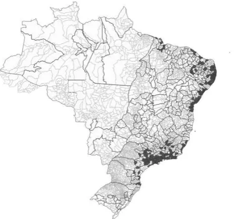
Figure 1 provides an overview of the result. It is notable that the further away from the sea, the larger the area of the municipalities. This pattern reflects the progressive populating process of an ex-colony emanating from the coast. The vast territory of many AMCs is thus not primarily related to the aggregation procedure but to the dimension of the municipalities in the interior. Four of them even have an area of over 100,000 sq km, which is larger than the territory of Portugal, for example. For areas of such dimension, it obviously makes no sense to estimate agglomeration economies, because they arise from the interaction between individuals within localized labor markets. It is thus necessary to limit the study to those AMCs that have the size of a coherent labor market. A reasonable number is 2,500 sq km. This corresponds to the area of a square with sides of 50 km, i.e.,
8
Reasons for the enormous increase in the number of administrative units are the expansion of the population and the economy and the political decentralization during the 1960s and 1970s (Reiset al.
2011).
9
an acceptable maximum distance to commute. Besides, this is also the average area of municipalities in the US.
[image:13.595.147.384.441.662.2]Because of these arbitrary restrictions and in view of the remaining AMCs (cf. the dark areas in figure 1) further comments are warranted. First of all, estimating the preferred specification (eq. (3)) in the sample with all AMCs – despite the concerns described above – yields qualitatively the same results that we present in the main text. Also, further tightening of the restriction on the AMCs’ areas does not change the fundamental insights of the paper. Considerations regarding the instruments also point out that the the area size restriction is preferable. Some AMCs are only vast because the municipality had a large territory in 1872. Even though nowadays a large city like Goiania, Brasília or Porto Alegre is contained in this vast AMC, the data does not reveal if and how far other settlements around that city influenced the value of the historical instruments. Obviously, Brasília did not even exist in 1872 or 1920 and thus the concentration of historical trades in whatever settlements existed within this AMC should not be used to predict the concentration of skills in Brasília in 2010. In any perspective, the accuracy of the instrument deteriorates undesirably with the AMC’s area. The descriptive figures in section 5.1 show that despite the area restriction, there is still extensive variation in population size and in the remainder of the essential variables exploited in this paper. These evaluations make us confident that the restriction to AMCs with an area of less than 2,500 sq km ultimately strengthens the credibility of the estimated agglomeration externalities.
Figure 1: Delineation of AMCs and municipalities
Notes: The figure shows the territory of Brazil to date. The fine lines indicate the borders of the munici-palities in the year 2010, whereas the bold lines mark the frontiers of the aggregated Minimum Comparable Areas (AMCs) for the period 1872–2010. Note that the territory of the Federal State Acre is excluded from our analysis because it was part of Bolivia in 1872. AMCs marked in dark are those with an area of less than 2,500 sq km. The observations from these AMCs define our sample.
4.3 Skills
Skill measures are the result of a division and systematization of individual activities in everyday work life. On the basis of the frequency and the intensity with which a specific skill/task is performed, occupations, and eventually workers, may be compared along a small number of skill dimensions. A further advantage of skills is that the distinction of workers according to their actual activities is more meaningful for some issues of economic analysis than, for example, their formal education. Skills/tasks recently found their way into labor economics and other related research fields through the work of Autor et al. (2003). They argue that technological progress in the form of IT, computers and automa-tion can replace routine and manual activities, whereas it complements analytical and cognitive skills. Consequently, one can also expect workers’ skills to play an important role in the analysis of agglomeration economies.
In Brazil, no workforce survey exists that assesses the skill/task requirements of workers in their occupations. Thus the only way to make progress is to adopt data from another country.10 One advantage thereof is that we can use established definitions which make
this study comparable to existing work. We tried several skill definitions, but throughout the study, we confine ourselves to two types of skills, to avoid duplicities and thus to save space. Following Acemoglu and Autor (2011) and Firpoet al. (2011), we distinguish between analytical and "face-to-face", i.e., interpersonal skills.11 To make the skill scores
comparable among one another, we standardize them to a mean of 10 and a standard deviation of 1 in the occupation data. Section A in the appendix provides a justification for the choice of these two skill measures alongside some numbers and graphs that relate the distribution of skills, occupations and wages. The observed pattern resemble those in the US or Germany.
5
Results
5.1 Descriptives
5.1.1 Concentration of skills
The current section provides an overview of the spatial distribution of the skill variables. This is interesting, not only because of the new definition of AMC regions, but also to verify whether Brazil exhibits patterns comparable to those of other countries.
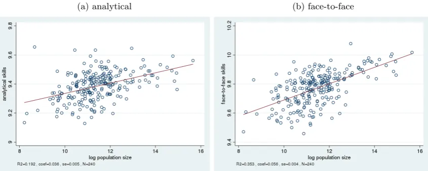
The vertical axis of the graphs in figure 2 denotes the concentration of the skill measures. This concentration is defined as the population-weighted average of a skill measure in the AMC. These averages vary between 9.2 and 9.9 in the case of analytic skills. It already
10
The assignment of an occupation characteristics survey to another country has been made previously. Anderssonet al. (2014), for example, transfer a German task classification into Swedish data, and Ehrl (2014b) relies on the same mapping between Brazilian jobs and US skills in a study about offshoring.
11
becomes evident that there are considerable differences in the vocational orientation of regions. Each scatter plot additionally reports the outcome of a simple unweighted OLS regression of the skill concentration on the log population per AMC. Both graphs show a clear pattern. The larger the size of the region in terms of population, the more analytical and face-to-face skill are performed in the local economy.12 The strength and explicative
[image:15.595.90.513.231.400.2]power of the regions’ size is somewhat higher for the concentration of face-to-face skills. Nevertheless, the robust standard errors confirm that both positive correlations are highly significant.
Figure 2: Spatial concentration of skills – AMC means
(a) analytical (b) face-to-face
Notes: The circles in each graph represent the AMCs’ skill averages and their log population size. Only AMCs with an area smaller than 2,500 sq km are part of the sample. The results from the corresponding (unweighted) linear regression are reported below each graph.
To get an idea of the dimension of the skill differences, consider the following stylized examples. São Luís do Quitunde in the Federal State of Alagoas in the North of Brazil has an average analytical skill value of 9.2 which is equivalent to a worker in a paper factory. In Florianópolis, in contrast, the capital of the State Santa Catarina in the South which has one of the highest analytic skill concentrations, an average occupation has the equivalent of a mechatronics technician or human resource analyst (9.6). In Areias (São Paulo), one of the smallest AMCs with only 3696 inhabitants, about 40% of the population make a living from agriculture and another 33% work in the construction or retail trade. The face-to-face skill index in Areias has a value of 9.47 which roughly corresponds to a worker in the construction sector. On the other side of the face-to-face skill distribution cities like Recife, Belo Horizonte and Rio de Janeiro have a value of about 10. Artists, like musicians or art directors, have just such an interactive skill score.
A similar overview for Brazil is provided in Maciente (2013). Although the definitions of the skills are different, namely less aggregated, and their alignment is by size groups of municipalities, it becomes clear that conclusions remain the same, that is to say, skills related to discipline, independence, attention or communication are more concentrated in
12
large municipalities.
5.1.2 Remuneration of skills
As a further motivation of our main analysis, we consider how the concentration of skills is related to the average wage level of a region. This time, both the plots and the univariate OLS regressions in figure 3 are weighted by the value of the population in the region. This representation is more important because it will be re-encountered in various wage regressions hereafter, which are estimated at the level of individuals.
As conjectured, regions where a disproportionately large amount of analytical and inter-active skills are executed have a substantially higher wage level, cf. figure 3. On the other hand, a concentration of manual skills, which can be particularly found in rural areas, is related to a lower overall wage level, cf. figure A.3 in Appendix B. Some AMCs are quite distant from the estimated regression line. These AMCs have an average of above 9.8 for interpersonal skills and at least 9.5 for analytical skills but at the same time they exhibit a very low wage level. A separate consideration reveals that these regions are predominantly rural and the high score in analytical skills stems from a large number of agricultural pro-ducers, agronomist, food scientists, etc. A robustness check in section 5.6.2 addresses this peculiarity.
How can those increasing regression lines be interpreted? On the one hand, one can imagine that the skill content of each occupation changes, without altering the region’s occupational composition per se. This is a counterfactual in which the daily work routine of every person is changed but admittedly it is less clear what the increase of skills by a certain value exactly means for each different profession. On the other hand, one could consider how the composition of occupations would have to change, to raise the value of the skill concentration in an AMC by a certain percentage, assuming the skills in each profession remained the same.
The difference of +1.0 in interpersonal skills equals the difference between a mechanical engineer or a wood technician and a manager (11.15 on average). So if everybody in a certain AMC would use this much more face-to-face skills, each wage would rise by 258%. This is certainly a high and unrealistic number, to the same extend as the large increase in interpersonal skills is unrealistic. Scaling the hypothetical increase in the average skill measure down to a less striking number of +0.01 thus implies average wage gains of 2.6%. Put differently, to raise the average face-to-face skill value of an AMC with a population equal to the mean (790,000) by 0.01, the region would have to experience an inflow of about 6,300 managers which corresponds to an increase of 8 managers per 1000 inhabitants.
Figure 3: Correlation between wages and concentration of skills – AMC means
(a) analytical (b) face-to-face
Notes: The circles in each graph represent the AMCs’ analytical and interpersonal skill and log wage averages using population weights. Only AMCs with an area smaller than 2,500 sq km are part of the sample. The results from the corresponding (unweighted) linear regression are reported below each graph.
5.2 OLS estimations
To make the descriptive observations about agglomeration economies in the previous sub-section more reliable, we propose two extensions. For one, we want to control for other wage determinants, such as education, age etc. It is thus more appropriate to consider wage regressions at the individual level. For another, we distinguish the effect of a spa-tial concentration of similar skills from other types of agglomeration economies, which, generically, may be captured by the size or density of the region (Rosenthal and Strange 2004).
The first column in table 1 shows the results from the estimation of eq. (1) where𝛽1 is set to 0, i.e., the effect of population size alone. The next two columns show the effect of the regional concentration of interactive skills without controlling for general agglomeration economies (𝛽2=0). Columns (4) and (5) include both of these variables and column (6) presents the results from the estimation of eq. (2). All of these estimations include our standard worker-specific controls as well as sector and state effects. Columns (3) and (5) additionally include occupation dummies. Virtually all of these control variables are highly significant and their coefficients are as expected. We report coefficients only for the most common and important variables. Wages increase monotonically in the education level, there is a slightly bell-shaped relation to the workers’ age and males earn more than observably equivalent females.
Table 1: Wage regressions on face-to-face skill measures
Dependent variable: log wage p.h.
(1) (2) (3) (4) (5) (6)
skill: AMC-level AMC-level AMC-level AMC-level individual
skill 0.748*** 0.661*** 0.177 0.119 0.166***
(0.073) (0.071) (0.143) (0.135) (0.009)
log(size) 0.070*** 0.061*** 0.057*** 0.068***
(0.004) (0.010) (0.010) (0.004)
skill*log(size) 0.043***
(0.004)
2.educ 0.011* 0.010* 0.009 0.010* 0.009* 0.013**
(0.006) (0.006) (0.005) (0.006) (0.005) (0.005)
3.educ 0.162*** 0.163*** 0.140*** 0.161*** 0.138*** 0.159***
(0.007) (0.007) (0.007) (0.007) (0.007) (0.007)
4.educ 0.353*** 0.353*** 0.274*** 0.352*** 0.273*** 0.335***
(0.010) (0.011) (0.008) (0.011) (0.008) (0.009)
5.educ 1.140*** 1.143*** 0.819*** 1.137*** 0.816*** 1.063***
(0.027) (0.029) (0.019) (0.029) (0.018) (0.023)
age 0.012*** 0.012*** 0.011*** 0.012*** 0.011*** 0.012***
(0.000) (0.000) (0.000) (0.000) (0.000) (0.000)
age2 −0.000*** −0.000*** −0.000*** −0.000*** −0.000*** −0.000***
(0.000) (0.000) (0.000) (0.000) (0.000) (0.000)
male 0.224*** 0.222*** 0.185*** 0.224*** 0.185*** 0.235***
(0.009) (0.009) (0.008) (0.009) (0.008) (0.009)
occ. dummies ✗ ✗ ✓ ✗ ✓ ✗
Constant 2.483*** 2.432*** 3.179*** 2.477*** 3.213*** 2.516***
(0.038) (0.047) (0.065) (0.038) (0.059) (0.039)
Obs. 1,293,046 1,293,046 1,293,046 1,293,046 1,293,046 1,293,046
R2 0.342 0.339 0.372 0.342 0.374 0.348
Notes: The skill variable in columns (2) to (5) is calculated as the weighted AMC average of face-to-face skills, whereas in column (6) the individual face-face-to-face skill value is used in the regression. Therefore, standard errors in brackets are clustered at the AMC-level in columns (2) to (5) and clustered at the AMC-occupation-level in column (6). Besides the variables shown in each row, the regressions also include dummies for sector, Federal State, occupational position, race, marital status, and whether or not the person is a foreigner, illiterate or has a physical deficiency. Regressions are weighted by the official sample weights provided by the Census. *denotes significance at ten, ** at five and***at one percent level.
agglomeration effect diminishes the strength of the general effect of size. However, the change here is small.
The last column in table 1 presents the estimation of eq. (2). The results also suggest that there are sizable agglomeration economies. The elasticity of wages with respect to population – evaluated for workers with face-to-face skill scores equal to the sample mean – (e.g. an actuary with a score equal to 9.8) is equal to 6.8%. The positive interaction coef-ficient in the third row indicates that the generic agglomeration effects rise, the higher the interpersonal skills of the worker and the larger the area’s population are. A worker with an interpersonal skill value of a standard deviation above the mean (executive directors for example who have a score of 10.9) has a by 4.1% higher wage elasticity. Altogether, these workers experience wage gains of 11.1% when the region’s population doubles, which corresponds to an increase of 63% compared to the elasticity of book keepers. This result suggests that interpersonal skills are necessary in order to capitalize the diverse agglomer-ation economies in large regions. These observagglomer-ations are in line with the literature on the importance of interaction in urban environments cf. Fujita and Thisse (2002). In particu-lar, our results are also quantitatively similar to those in Bacolodet al.(2009a: 145). Using US data, those authors obtain a (plain) wage elasticity with respect to population of 4.4% and workers "with the ability to interact" also have a more than 50% higher elasticity.13
The extent to which the entire population or only some groups benefit from the spillovers is investigated in subsection 5.5.
5.3 Basic IV results
Our instrumental variable strategy intends to identify the unbiased and causal effect of an agglomeration of interpersonal skills on wages. The assumption underlying the identifica-tion strategy is that the occupaidentifica-tional structure of a region 140 or 90 years ago has been shaping the further economic development of that region until the present day. In partic-ular, a high concentration of industrialists and liberal professions has fostered a positive long-run development which has resulted in a conglomeration of high-skilled jobs, which largely require those interactive (and analytical) skills.
Section 3 described how both education and manufacturing production in factories were scarce and hence quite valuable at the turn of the 19th
century. Moreover, it is likely that lawyers and judges, who are also part of the liberal professions served to stabilize the fragile institutions, maintain law and order and guarantee property rights, all essential conditions for investment and economic growth (Acemogluet al.2001). The composition of the local economy was much more important than nowadays because railroads had still hardly been built and hence overland transport costs were high. This constellation favored economic development in those regions where the seed for knowledge and industrial production was already sown, whereas regions shaped by agriculture and slavery were likely to remain locked-in and without impulses towards modernization.
Figure 4 illustrates our identifying assumption. The upper left graph of figure 4 shows
13
that the proportion of industrialists in 1872 explains 19% of the spatial dispersion of interpersonal skills in 2010. The coefficient of this linear regression – stated below the graph – is highly significant and indicates that doubling the number of industrialists in a region is associated with a 0.05 (or 1
[image:20.595.97.501.243.537.2]2 standard deviation) higher face-to-face skill index. The relation is much weaker regarding the share of the liberal professions in 1872. In this linear regression, the instrument has to be classified as weak. This assessment definitely changed 48 years thereafter. Now the explained percentage of 55% is also higher than that of the manufacturing sector. Regarding analytical skills a very similar picture emerges; compare supplementary figure B.1.
Figure 4: Correlation between face-to-face skill mean and historical trades
Notes: The circles in each graph represent the AMCs’ interpersonal skill average and each one of the four instrumental variables in the sample. The results from a weighted linear regression of each of the IVs on the face-to-face skill concentration are indicated below each graph.
It is certainly impossible to pin down a single channel through which history has shaped the present. Yet figure 4 suggests that our instruments go a long way towards explaining the long-run industrial development of regions. The data also show that the less far we look into the past, the stronger becomes the relation to the previous occupational composition, albeit the structure of the economy has still changed significantly over the last 90 years. The following tables deepen the interpretation and the exploration of the relevance and exogeneity of our instrumental variables.
Table 2 show the results from the estimation of eq. (3) where the concentration of face-to-face skills is instrumented.14 The set of exogenous individual and sectoral control variables
14
is the same as in previous estimations, cf. table 1. Again, by means of occupation fixed effects we also account for the fact that the actual professions of workers also affect wages. The first column repeats the OLS coefficient for comparison. In the next four columns, each one of our historical IVs is used. Then, both IVs from 1872, and 1920, respectively are used jointly. The last two columns show the results when all four instruments are applied simultaneously. In the lower part of the tables, the corresponding coefficients of the IVs from the first-stage regressions are presented along with other statistics that allow for the assessment of the IVs’ performance.
[image:21.595.92.530.388.644.2]By and large, the same picture emerges as described by means of the four simple regres-sions in figure 4. Considered separately, all instruments’ coefficients are significant at the 1% level in the first stage regressions. The magnitude of these coefficients is similar to the one identified in the univariate regressions beforehand, and the interpretations of the coefficients apply equally. When considered jointly, only one or two of the instruments re-main significant in table 2. Based on the univariate scatter plots, we were already able to foresee which one dominates. For 1872, the concentration of industrialists has the strongest effect on the concentration of analytic skills, whereas for 1920, the concentration of liberal professions is the more powerful instrument.
Table 2: Basic IV regressions – face-to-face skill concentration
Dependent variable: log wage p.h.
OLS IV (1) IV (2) IV (3) IV (4) 1872 IVs 1920 IVs all IVs all IVs face-to-face 0.661*** 0.765*** 0.898*** 1.066*** 1.064*** 0.854*** 1.064*** 1.086*** 1.004***
skill conc. (0.071) (0.173) (0.159) (0.108) (0.092) (0.153) (0.092) (0.087) (0.086)
1.-stage statistics
1872: log of 0.062*** 0.045*** 0.012 0.012
ind. per 1000 (0.012) (0.013) (0.012) (0.012)
1872: log of 0.044*** 0.017* 0.005 0.004
liberal per 1000 (0.010) (0.010) (0.009) (0.009)
1920: log of 0.087*** 0.022 0.019 0.020
ind. per 1000 (0.009) (0.014) (0.013) (0.014)
1920: log of 0.093*** 0.075*** 0.069*** 0.068***
liberal per 1000 (0.006) (0.011) (0.012) (0.012)
1. R2-part. 0.182 0.152 0.409 0.487 0.191 0.493 0.507 0.462
weak IV: F 26.900 20.750 106.100 213.100 18.860 105.800 53.390 44.400
weak IV:τ=5% 37.420 37.420 37.420 37.420 19.040 13.320 20.960 20.810
weak IV:τ=10% 23.110 23.110 23.110 23.110 12.310 8.947 12.730 12.640
weak IV:τ=20% 15.060 15.060 15.060 15.060 8.462 6.418 8.214 8.160
weak IV:τ=30% 12.040 12.040 12.040 12.040 6.994 5.453 6.558 6.518
K 1.316 12.730 7.432 5.207
K-p 0.251 0.000 0.006 0.023
Hanson J 1.194 0.001 3.598 3.474
Hanson J-p 0.275 0.972 0.308 0.324
Notes: The regressions control for a quadratic in worker’s age, dummies for occupation, sector, Federal State, education level, occupational position, race, marital status, and whether or not the person is a foreigner, male, illiterate or has a physical deficiency, is as specified before. All regressions are weighted by the Census population weights. The estimation in the last column additionally includes the 1𝑠𝑡
nature advantage proxies. Standard errors in brackets are clustered at the AMC-level. The number of observations varies slightly due to few missing values of the IV but it lies above 1,290k in all of the estimations. *denotes
significance at ten,** at five and*** at one percent level.
The main novelty from these IV regressions compared to the OLS regressions in table
1 is that the effect of the instrumented skill variable is now larger. The effect of the interpersonal skill concentration lies between 0.8 and 1.1. We conclude that measurement error and endogeneity bring about some substantial bias of the agglomeration effects of skill concentrations estimated by OLS. Using instrumental variables, the skill concentrations have a significant and positive effect throughout all estimations here. The weak IV statistics based on Stock and Yogo (2005) demonstrate that these coefficients, particularly when two or all four IVs are used, are estimated with a bias of less than 5–10%. The K statistic provides another way of testing the relevance of the instruments. It also reflects the critical view of the 1872s instruments. For the 1920s IVs and the joint estimations, however, it clearly underscores their high predictive power. Hansen’s J statistic, however, offers a uniform picture. Wherever it is possible to perform the overidentification test, the IVs’ exogeneity clearly cannot be rejected.
The last column in table 2 repeats the estimates with all four IVs but additionally includes controls for1st
nature advantages. Of course, the distance to the nearest coastline has not changed over time. But also the number of railway stations after the peak of its construc-tion activity has remained relatively constant until the present day. If settlement decision by industrialists and people with liberal professions as well as the long-run economic de-velopment up to the skill distribution in today’s industries were substantially affected by those1st
nature advantages, then the coefficients and in particular the explanatory power of our IVs should differ clearly from the previous estimates. Note that these estimations represent our preferred specification because all IVs are used simultaneously and we control for the maximum number of exogenous variables.
As expected, the distance to the coast shows a negative but insignificant sign in the second stage regression and the number of railroad station has a positive and significant correlation with wages (not shown in the tables). Yet the results remain almost unchanged. Both the first stage coefficients of our IVs and the instrumented coefficient of the skill variable are close to the estimates in the previous column. Even the partial 𝑅2 of the IVs in the
first stage regression is not changed much. We therefore conclude that distance from the coastline and the railroad transport system may represent a productivity advantage even today, but their existence has not affected the distribution of historical professions in a crucial manner. Thus, the exogeneity of our IVs is confirmed once again.
The coefficient in our preferred estimation indicates that an increase in the face-to-face skill index by one standard deviation (equal to 0.1) results in an average wage increase of 10%. To induce this change of +0.1, a region with a population and skill index equal to the sample mean would require an inflow of +88 managers per 1000 inhabitants, for example. This true effect of interpersonal skills is thus much smaller than the one conjectured from the simple OLS regression without any control variables in figure 3.
5.4 IV estimation with different size groups
that the wage externalities increase with the size of the region. Since current population is an endogenous variable, too, pursuing this strategy further would mean to instrument two endogenous variables plus their interaction term. Estimating and interpreting such a model with interaction of instruments is beyond the scope of the paper. A feasible possibility is to split the sample into groups based on the size of the regions and to estimate the effects within those separate subsamples.
At the same time, and even more importantly, we can perform another investigation with this regional distinction. Our hypothesis is that the long-run development of regions cru-cially depended on their initial size. In particular, we rely on New Economic Geography theories, which address the attractiveness of agglomerations and the process of their forma-tion. Up to here, our historical instruments show that the concentration of knowledge and manufacturing has led to a continuous modernization and finally to a higher concentration of high-skilled occupations. However, it could be that this supply-side agglomeration is just a necessary but not a sufficient condition for a sustainable growth path. In line with the initial quote by von Thünen, New Economic Geography teaches that circular causality between demand and supply side promotes the growth of regions and guarantees their continuous attractiveness for workers and firms. This means that if a region was blessed with a sufficiently large number of customers for fabricated products and people who make use of the locally available knowledge, this region would experience higher growth rates than small regions. Consequently, regions with such favorable characteristics in the past should have a greater concentration of high-skilled occupations that predominantly require analytical and interpersonal skills.
5.4.1 Definitions of AMC groups according to population size
Following the theoretical arguments above, we divide the AMCs according to their pop-ulation size in 1872 or 1920 into two groups each. AMCs in the "Large" group have a population above the median in the distribution of AMCs. Consequently, the other half of the AMC in the "Small" group has a lower population. We prefer this specific division because dividing the sample according to the population weighted mean, for example, gives approximately the same number of people in both groups, but the number of AMCs in the "Large" group becomes very low. Given that the number of AMCs with an area of less than 2,500 sq km amounts to no more than 240 and the main variables of interest only have variations between AMCs, the division according to the median is the best option that allows for a reasonable identification of the effects in both groups.
the density distributions in 1872 of theSmall size group are slightly skewed to the right. This pattern is reversed in 1920. Although it is rather natural that a higher concentration of liberal professions are to be found in more populated areas, the density distributions are quite close to each other in both size groups for liberals and industrials, respectively. Hence, from this point of view, no significant systematic differences are to be expected in the following IV regressions between the defined agglomeration groups. Note that this fact cannot be inferred from the summary statistics in table B.1 because the table shows weighted values.
Figure 5 shows the dispersion of AMCs across all four agglomeration groups as well as the the development of the AMCs’ population over time. Each of the three scatter plots shows the size of the AMCs in either 1872 or 1920 on the axes. The vertical and horizontal straight lines denote the median of the variable on the respective axis, which is exactly the value that classifies AMCs asLarge or Small. The drawn 45∘ line serves as an orientation
as to whether and how much a region has grown. All of the three graphs indicate that some AMCs with below average population, have grown substantially and climbed into the higher size class, while the contrary is also visible. These transitions are unsurprisingly more frequent the larger the considered period is. Certainly, the size of regions is highly persistent, however the transitions of AMCs between the different groups confirm that there is room for explanations as to why a region has taken either a good or an unfavorable growth path.
5.4.2 IV results for AMC size groups
Table 3 present the estimations after the division of the sample according to the agglom-eration groups defined above. We report OLS and IV estimates for the face-to-face skill concentration. In the first two columns, we split the sample according to the AMC’s size in 1872 and consequentially only apply both instruments from 1872. Analogously, columns (3) to (4) refer to one of the 1920’s size groups and include the two IVs from 1920 in-stead. Each estimation contains the full set of control variables, including the 1st
nature advantage controls. Because the number of clusters is close to the number of regressors (72) in these GMM estimations, we had to partial out some variables (the UF dummies) in order to obtain weighting matrices of full rank. By the Frisch-Waugh-Lovell theorem, the remaining coefficients are unchanged, however (Baum et al.2007). Yet Stock-Yogo weak IV statistics cannot be calculated and we resort to the simple 1. stage F-value.
Three patterns stand out. First, no matter which of the two group definitions is used, in each IV estimation, only the skill concentration for the largest group shows a significant coefficient at the 1% level. Second, these coefficients are comparable to the previous IV estimations. In fact, the coefficient from the estimation with the 1872 IVs is somewhat lower than in table 2 but, as we have seen previously, this coefficient is estimated with less precision than those in the IV regressions with the IVs from 1920.
Figure 5: Development of AMCs across size groups
Notes: The circles in each graph represent the AMCs’ population in different years. The vertical and horizontal straight lines denote the median of the variable on the respective axis, i.e., the value that divides the AMCs in the sample into the group ofLargeorSmall AMCs. The dashed lines represent a 45∘line through the origin.
at the 1% level which, however, cannot be confirmed in the IV estimation. This obser-vation suggests that agglomeration economies arise only in highly populated regions and, conversely, externalities are not significantly measurable in regions with sparse population. So it seems that there is a kind of ‘critical mass’ for the occurrence of these externalities.
The third pattern concerns the relevance of the instruments. Only in the group of the most populated AMCs is there a substantial relation between the concentration of face-to-face skills and the supply of manufacturing and liberal professions in the previous century. Note that in table 3 both𝑅2 and the first-stage F-values are close to zero for the Small AMCs. In contrast, these first-stage statistics in the group of theLarge AMCs are satisfactory and even higher than in the full sample. Only the K statistic indicates paradoxically that the 1872 IVs are weak, even though the first stage F-value amounts to 23. These facts also explain why a significant externality is identified only for this group. As before, the results for the analytic skill concentrations are relegated to the appendix (table B.3) but follow the described pattern of the face-to-face skill concentration.
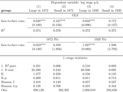
observa-Table 3: IV regressions – agglomeration groups – face-to-face skills
Dependent variable: log wage p.h.
(1) (2) (3) (4)
group: Large in 1872 Small in 1872 Large in 1920 Small in 1920
OLS
face-to-face conc. 0.628*** 0.447*** 0.632*** 0.172 (0.100) (0.156) (0.090) (0.127)
R2 0.374 0.376 0.372 0.375
1872 IVs 1920 IVs
face-to-face conc. 0.653*** 0.850 1.027*** 1.506 (0.130) (1.956) (0.088) (5.792)
1.-stage statistics
1. R2-part. 0.351 0.006 0.516 0.003 1. F-stat 23.280 0.242 68.930 0.095
K 1.577 0.259 6.550 0.135
K-p 0.209 0.611 0.011 0.713
Hanson J 2.318 0.140 0.857 0.587
Hanson J-p 0.128 0.708 0.355 0.444
Obs. 898,139 392,305 1,000,010 293,036
Notes: The sample is split according to the median AMC population size in 1872 and 1920 in columns (1), (2) and (3), (4), respectively. All regressions include the basic control variables specified in table 2 and the1𝑠𝑡
nature advantage proxies. Regressions are weighted by the Census population weights. UF dummies are partialed out due to the high number of exogenous variables relative to the number of clusters. Standard errors in brackets are clustered at the AMC-level. * denotes significance at
ten,** at five and***at one percent level.
tion provides an indication about the mechanism by means of which industrial and liberal professions have transformed into modern industries over time. Interaction between sup-ply (factories) and consumer demand (population) created a virtuous cycle for the local economy. In a wider perspective our findings suggest that market potential and history do play a crucial role in the development of agglomerations, as argued by theories of the New Economic Geography.
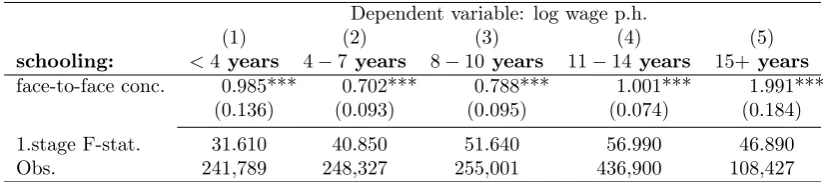
5.5 Heterogeneous effects
As a last extension, we analyze whether the agglomeration effects are heterogeneous in different segments of the population. So far we have seen that workers generate more or less pronounced spillovers in accordance with their professional activity. Likewise, workers may also differ as recipients of these spillovers.
[image:26.595.92.505.95.405.2]