The E Monetary Theory

Munich Personal RePEc Archive

The E-Monetary Theory

Ngotran, Duong

SUNY Albany

10 October 2016

Online at

https://mpra.ub.uni-muenchen.de/84940/

The E-Monetary Theory

∗

†

Duong Ngotran

First Version: Oct, 2016. This Version: Jan, 2018

University at Albany, State University of New York

Abstract

We develop a dynamic model with two types of electronic money: reserves for transactions be-tween bankers and zero-maturity deposits for transactions in the non-bank private sector. Using this model, we assess the efficacy of unconventional monetary policy since the Great Recession. After quantitative easing, keeping the interest on reserves at zero too long will create deflation. The central bank can safely get out of the “low rate-cum-deflation” trap by “raising rate and raising money supply”.

JEL codes: E4, E5

Keywords: interest on reserves, quantitative easing, unwinding QE, e-money, excess

re-serves, raise rate and raise money supply

∗_{I would like to thank Adrian Masters for his guidance and support during this project. Special thanks to Betty}

Daniel, Michael Sattinger, Michael Jerison for helpful comments and discussions. I also thank to Yue Li, Ibrahim Gunay, Savita Ramaprasad, Minhee Kim, Garima Siwach, Kang Gusang, Tu Nguyen and other participants in Midwest Macro Meeting and AEA Poster Session. All errors are my own.

†_{This paper is a substantial revision ofNgotran(2016). The model is streamlined due to helpful comments of}

1

Introduction

Nowadays, money mostly exists in the electronic form. According to data from the Federal

Reserve Bank of St. Louis, the total stock of M1 in Jun 2016 is around USD 3274 billion,

con-sisting of USD 1381 billion in currency and USD 1850 billion in checkable deposits. However,

as the world currency, most US dollar bills are held outside US.Judson(2012) estimates that 60 percent of US dollar bills are in foreign countries. If we exclude that number from M1 and

M2, currency only accounts for 23 percent of M1, 5 percent of M2 and 4.2 percent of MZM1.

In this paper, we focus on a popular group of e-money issued by commercial banks, including

checkable deposits, saving deposits and money market deposit accounts. Together they account

for 80 percent of M2. For convenience, we call this group as zero-maturity deposits (ZMDs)

thereafter.

ZMDs are different from currency in two salient features. First, in nature, currency is an

IOU issued by the central bank while ZMDs are IOUs issued by commercial banks. In the

lan-guage of economics, currency is outside money while ZMDs are inside money. Second, in the

households’ perspective, unlike currency, ZMDs can earn nominal interest. Banks pay interest

for saving accounts and money market deposit accounts for a long time, but the tricky parts are

checking accounts. In a perfectly competitive banking market, the interest rate on checkable

deposits should be positive and follow the federal funds rate2. However, before 2012, under the

Regulation Q, banks in US were prohibited from paying interest on checking accounts. During

this period, banks still implicitly paid the demand deposit rate under the form of NOW

(nego-tiable order of withdrawal) accounts, giving gifts or reducing the cost of additional services to

their customers, see Mitchell (1979), Startz (1979), Dotsey(1983). Becker (1975) estimates that the implicit demand deposit rate in US during 1960-1968 was around 2.64 percent to 3.74

percent.

Since 2012, the Regulation Q has been no longer valid, and most banks are now paying

interest rate on checkable deposits. Data in September 2016 of Federal Deposit Insurance

Cor-1_{MZM (Money zero maturity) is equal to M2 less small-denomination time deposits plus institutional money}

funds.

poration (FDIC) show that the national average interest on checkable account is 0.04 percent,

on saving account is 0.06 percent. These rates are low as the federal funds rate is near zero. If

the federal funds rate is around 4 percent, these rates are likely from 1 percent to 2 percent. As

a result of that, in the era of electronic money, it is more natural to model money as an

interest-earning asset that provides liquidity service.

This paper builds a dynamic general equilibrium model where currency does not exist (a

cashless model). There are two forms of money in our model: ZMDs and reserves. ZMDs

are inside money issued by commercial banks. They are used for settling transactions between

every pair of agents in the private sector, except between bankers-bankers. In these types of

transactions, bankers have to use reserves- another type of e-money that is issued by the central

bank. The amount of ZMDs that banks can issue is restricted by two constraints: the reserves

requirement and the capital requirement. In our model, the central bank only controls the level

of reserves while the level of the money supply (amount of ZMDs) depends on the interaction

between the central bank, the commercial banks and the public (Mishkin,2007).

We use our model to discuss unconventional monetary policy during and after the Great

Recession. Here are some key results:

i. In normal times, when the central bank controls the federal funds rate by adjusting the level

of reserves, the effect of cutting rates in our model is nearly identical to the one founded

in the standard New Keynesian model. After the interbank rate goes down, the real rate

goes down as price is sticky. Banks lend out more to households by creating more money

(Sheard,2013), stimulating inflation and investment.

ii. After a shock that makes banks’ capital constraint binding, an interest rate policy following

a Taylor rule is not enough to recover the economy quickly. Both output and inflation are

lower than their steady state levels for a long time.

iii. A central bank’s large scale asset purchase (LSAP) program, with the aim of directly

in-jecting money into the economy, is very efficient at dealing with the situation when bankers

the reserves requirement is no longer binding; and interest on reserves (IOR) becomes the

main tool to control the federal funds rate.

iv. After LSAP, the longer the federal funds rate is committed at the lower bound, the higher

is inflation in the short run. As loans have the longer maturity than deposits, commitment

to keep the short-term rate near zero for a long time pushes down the loan rate stronger.

However, in the long run, it might create a persistent deflation due to the Neo-Fisherian’s

effect. The real short-term rate will slowly climb back to the long-run level. The

endoge-nous money supply declines, and deflation realizes. This matches with the US data since

the Great Recession (Figure1).

v. It is not easy to safely escape from the “low rate-cum-delfation” trap. If the central bank

raises rates (by raising IOR), the amount of banks’ credits declines. The economy will

suffer a short recession. Deflation is even more severe in the short run. However, inflation

will jump back to the target in the long run. Therefore, the central bank falls into a dilemma

between to raise or not to raise rates. Either way the outcome is not bright.

vi. When raising IOR, if the central bank simultaneously commits to target the growth rate of

the money supply in response to inflation, the inflation and output path will be stabilized.

In the electronic payment system, the central bank somehow can manipulate both interest

rate and money supply at the same time. These tools should be utilized simultaneously so

that the central bank can hit the inflation target better.

Related Literature

On the money supply side, our approach is similar toBianchi and Bigio(2014) andAfonso and Lagos (2015) when the central bank can increase the level of the money supply and cut down the federal funds rate by injecting more reserves in the banking system. These papers

ex-plicitly model the search and matching process of heterogeneous agents in the interbank market

while our model is frictionless with identical bankers. On the other hand, our model can connect

the central bank policy to not only banks’ balance sheet but also the production sector, which is

-­‐2.0   -­‐1.0   0.0   1.0   2.0   3.0   4.0   5.0  

0.00   1.00   2.00   3.00   4.00   5.00   6.00  

2007-­‐01-­‐01   2007-­‐06-­‐01   2007-­‐11-­‐01   2008-­‐04-­‐01   2008-­‐09-­‐01   2009-­‐02-­‐01   2009-­‐07-­‐01   2009-­‐12-­‐01   2010-­‐05-­‐01   2010-­‐10-­‐01   2011-­‐03-­‐01   2011-­‐08-­‐01   2012-­‐01-­‐01   2012-­‐06-­‐01   2012-­‐11-­‐01   2013-­‐04-­‐01   2013-­‐09-­‐01   2014-­‐02-­‐01   2014-­‐07-­‐01   2014-­‐12-­‐01   2015-­‐05-­‐01   2015-­‐10-­‐01  

PCE  

FFR  

FFR   Infla4on   Infla4on  Target  

Figure 1: Federal Funds Rate and Personal Consumption Expenditure Index

On the money demand side, our model follows the cash-in-advance approach inLucas and Stokey (1987). As our model does not have currency, “cash” here should be interpreted as ZMDs. InBelongia and Ireland(2006, 2014), currency and deposits are bundled together and provide the liquidity service to households. We also extend the Clower constraint to investment

(Stockman(1981),Abel(1985),Fuerst(1992),Wang and Wen(2006)). Indeed, most empirical research, for exampleFriedman(1959) andMulligan and Sala-I-Martin(1997), usually uses the income, rather than the consumption alone, to estimate the money demand function.

Our model is still in the general New Keynesian framework with the crucial sticky price

fea-ture. The important role of financial frictions in the New Keynesian has been emphasized for a

long time (seeBernanke, Gertler and Gilchrist(1999),Christiano, Motto and Rostagno(2004)). Recently, many New Keynesian research (Gertler and Kiyotaki(2010), Curdia and Woodford

(2011), Gertler and Karadi(2011)) incorporates the banking sector to their models, aiming to answer what happened in the Great Recession and the role of the unconventional monetary

pol-icy. There is also a large literature that discusses interest on reserves, seeSargent and Wallace

(1985), Goodfriend et al.(2002), Ireland(2014), Cochrane(2014), Keister (2016). Our paper differs mainly from this line of research in the money supply process. We can characterize the

micro-foundation link between bank reserves, banks’ balance sheets, money supply, interest rate

and output. We emphasize the importance of both money supply and interest rate in monetary

affect strongly to the balance sheets of intermediaries and the amount of inside money. Both

papers emphasize the importance of inside money in the deflation episode. However, two papers

differ mainly in the role of money and the money supply process. They emphasize the money

function as a store of value in a risky environment while our paper focus on the common role of

money - medium of exchange - in a deterministic setting.

2

The Environment

2.1

Notation:

LetPt be the price of the final good. We use lowercase letters to represent the real balance of a

variable or its relative price to the price of the final good. For example, the real reserves balance

nt =Nt/Pt, or the relative price of the intermediate good to the final good is pmt =Ptm/Pt. The

timing notation follows this rule: if a variable is determined or chosen at timet, it will have the

subscriptt. The gross inflation rate isπt=Pt/Pt−1.

2.2

Time, Demographics and Preferences

Time is discrete, indexed byt and continues forever. The model is in the deterministic setting

and has five types of agents: bankers, households, wholesale firms, retail firms, and the

consol-idated government.

There is a measure one of identical infinitely lived bankers in the economy. Bankers

dis-count the future with the disdis-count factorβ. Each period, they gain utility from consuming the

final consumption goodct. Their utility at the periodt can be written as:

∞

∑

βilog(ct+i)

There is also a measure one of identical infinitely lived households. Households discount

the future with the discount factorβe<β, so they will borrow from bankers in the steady state.

utility when providing laborlt to their own production. Household’s utility at the periodt can

be written as:

∞

∑

i=0

e

βi log(c˜t+i)−χ l

1+ν t+i

1+ν !

whereν is the inverse Frisch elasticity of labor supply.

Wholesale firms, retail firms are infinitely lived, owned by households.

The consolidated government includes both the government and the central bank, so for

convenience, we assume there is no independence between the government and the central bank.

2.3

Goods and Production Technology

There are three types of goods in the economy: final goodyt produced by retailers, wholesale

goodsyt(j)produced by wholesale firm jand intermediate goodym_t produced by households.

Each period households self-employ their labor lt and use the capital kt−1 to produce the

homogeneous intermediate goodym_t under the Cobb-Douglas production function:

y_tm=kα_t−1l_t1−α

whereαis the share of capital in the production function. Capitalkdepreciates with the rateδk.

Households also own a technology to convert one unit of final goodytto one unit of capital type

kand vice versa. So each period they also make an investmentit=kt−δkkt−1. Households sell

y_tmto wholesale firms in the competitive market with priceP_tm.

There is a continuum of wholesale firms indexed by j∈[0,1]. Each wholesale firm purchases

the homogeneous intermediate goodym_t from households and differentiates it into a distinctive

wholesale goodsyt(j)under the following technology:

Then retail firms produce the final goodyt by aggregating a variety of differentiated

whole-sale goodsyt(j):

yt =

Z 1

0

yt(j)ε−1ε _{d j}

ε

ε−1

2.4

Assets

There are three main types of financial assets (excluding reserves and deposits): bank loansBh_t,

share of wholesale firmsxt and interbank loansB_tf.

(a) Bank loans to households (Bh_t): We followLeland and Toft(1996) andBianchi and Bigio

(2014) to model the loan structure between bankers and households. The market for bank loan is perfectly competitive and the price of loan isq_tL. When a household wants to borrow

1 dollar at timet, bankers will create an account for her and depositq_tLdollars to her account.

In the exchange for that, this household promises to pay δb, δ_b2, ..., δ_bn, δ_bn+1... dollars at

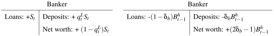
timet+1,t+2,... t+n, t+n+1... where nruns to infinity (Table1). Loans are illiquid and bankers cannot sell loans.

Let B_th be the nominal balance of loan stock in the periodt, let St be the nominal flow of

new loan issuance, we have:

Bh_t =δbBht−1+St

(b) Shares of wholesale firms (xt): are issued by the wholesale firms. Bankers are not allowed

to hold this share, so they are only traded between households. Each share has a price υt

and pays a real dividendwt. The number of wholesale firms’ shares is 1. In the LSAP, the

central bank might purchase these shares to inject money into the market.

(c) Interbank loan (B_tf): Bankers can borrow reserves from other bankers in the federal funds

market. The nominal gross interest rate in the federal funds market is the federal funds rate

Banker Banker

Loans: +St Deposits: +qLtSt Loans: -(1−δb)Bh_t−1 Deposits: -δbBh_t−1

Net worth: +(1−q_tL)St Net worth: +(2δb−1)Bt−h 1

Table 1: Banker issues loans (left) and collects loans (right)

2.5

Money

There are two types of electronic money in our economy: reservesnt and zero-maturity deposits

mt.

(a) Reserve (nt): is a type of e-money issued by the central bank. Only government and bankers

have an account at the central bank, so only government and bankers have reserves3. Each

period, the central bank pays a gross interest rate Rn_t on these reserves. The rate R_tn is

decided solely by the central bank. Reserves are used for settling the transactions between

bankers and bankers, bankers and central bank, bankers and government.

(b) Zero maturity deposit (mt): is a type of e-money issued by bankers. Each period, banks

pay the interest rateRm_t for these ZMDs which is determined by the perfectly competitive

market. Money mt is used for settling transactions in the non-bank private sector and the

ones between households and bankers. These ZMDs are insured by the central bank, so

they are totally safe. ZMDs and reserves have the same unit of account.

In the electronic payment system, there is a connection between the flows of reserves and

de-posits. For example, we assume that wholesale firm A (whose account at bank A) pays 1 dollar

for household B (whose account at bank B). Then the flow of payment will follow Table (2). For a transaction between the consolidated government and households, money still flows through

banks, so we can think that this contains two sub-transactions. One is between the government

and banks, which is settled by reserves. One is between banks and households, which is settled

by ZMDs.

In the conventional monetary policy, the consolidated government targets the interbank rate

3_{The amount of US Treasury deposits at the Fed is not considered as reserves in reality. However, for}

Wholesale firm A Household B

Deposit: -1 Payable:-1 Deposit: +1

Receivable:-1

Bank A Bank B

Reserve: -1 Deposit: -1 Reserve: +1 Deposit: +1

The Fed

Reserve (bank A): -1

Reserve (bank B):+1

Table 2: Electronic Payment System

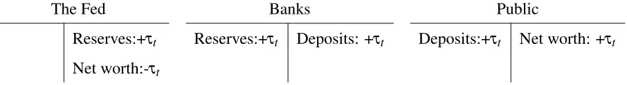
by helicopter money or lump-sump tax on households. Each period, the central bank sendsτt

dollars in checks to households. It can be thought as a shortcut of the open market operation

pro-cess when the central bank purchases government bonds from the government (through banks).

Then, the government transfers the payoffs to households (Table3). In fractional reserve bank-ing, the amount ofτt needed to change the federal funds rate is extremely small in comparison

to the total money supply.

The Fed Banks Public

Reserves:+τt Reserves:+τt Deposits: +τt Deposits:+τt Net worth: +τt

Net worth:-τt

Table 3: Helicopter Money / Lump-sum tax

2.6

Timing within one period

(i) Production takes place. Households sell goods to wholesalers, who, in turn, sell goods to

retailers. All of the payments between households-wholesalers, wholesalers-retailer are

delayed until the step (iv).

(iii) The final good market opens. Households need ZMD-in-advance to purchase the final

good from retailers. Bankers create ZMD to purchase the final good from retailer.

(iv) Payments in the non-bank private sector are settled.

(v) The banking market opens. Banker can adjust the level of reserves by borrowing in the

interbank market, receiving new deposits.

3

Agents’ Problems

3.1

Bankers

There is a measure one of identical bankers in the economy. These bankers have to maintain a

good balance sheet under the regulation of the central bank. There are three types of assets on a

banker’s balance sheet: reserves (nt), loans to households (bht), loan to other bankers (b f t). His

liability side contains the zero-maturity deposits that households deposit here (mt).

Banker

Reserves: nt Zero Maturity Deposits: mt

Loans to households: bh_t Net worth

Loans to other bankers:b_tf

Cost: We assume that the banker faces a cost of managing loan, which isθbh_t in terms of

final goods.

On the timing of the market, it is worth noting that he can adjust the level of his deposits

and reserves after households and firms pay for each other. When the different parties in the

economy pay each other, he can witness that the deposits and reserves outflow from or inflow

to his bank. Letet be the net inflow of deposits and reserves go into his bank, he will treatet

exogenously. When the banking market opens, as the deposit market is perfectly competitive,

he can choose any amountdt of deposit inflows or outflows to his bank.

to maximize his utility over a stream of consumptions:

max

∞

∑

t=0

βtlog(ct)

subject to

Rn_t−1nt−1

πt +

R_t−f ₁b_t−f ₁

πt +dt+et+τt =nt+b

f

t (Reserve Flows) (1)

mt=

Rm_t−1mt−1

πt

+qL_tst+θbth−δb

bh_t−1 πt

+ct+dt+et+τt (Deposit Flows) (2)

bh_t =δb

b_t−h ₁

πt +st (Loan Flows) (3)

nt≥ϕmt (Reserves Requirement) (4)

nt+btf+bht −mt ≥κtbth (Capital Requirement) (5)

Reserve Flows: in each period are shown in the equation (1). After receiving the interest on reserves, the previous reserve balance becomesRn_t−1nt−1/πt. He also collects the payment

from the interbank loan he lends out to other bankers in the previous periodR_t−f ₁b_t−f ₁/πt. He

can also increase his reserves by taking more depositsdt. When doing that, his reserves and

his liability increase by the same amountdt (Table 4). That is the reason we seedt appear on

both the equation (1) and (2). The similar effect can be found onτt when the central bank drops money. The banker treatsτt exogenously. Then, he can leave reservesnt at the central bank’s

account to earn interest rate, or lend reserves to another bankersb_tf.

Deposit Flows: for the banker are shown in the equation (2). He makes loans to households by issuing deposits or creating ZMDs (Table1). So when he makes a loan (st), the balance sheet

expands. When he collects the payoffs from loans to households (δbbh_t−1/πt), the balance sheet

shrinks4.

The banker also issues his own ZMDs to purchase the consumption good from retailers (ct)

and to pay for the cost (in terms of final goods) related to lending activities (θb_th) (Table4). It is

4_{It is assumed that households have to pay loans from the account at the bank they borrow. So if they want to}

Banker Banker

Reserves: +dt Deposits: +dt Reserves: -btf

Interbank loan: +b_tf

Table 4: The banker takes more deposits (left) and makes interbank loan (right)

Banker Banker

Deposits: +ct Deposits: +θbh_t

Net worth: -ct Net worth: -θbht

Table 5: The banker pays for his consumption (left) and pays for cost (right)

noted that he cannot create infinite amount of money for himself to buy consumption goods as

there exists the capital requirement.

Reserve Requirement: At the end of each period, he has to hold enough reserves as a

fraction of total deposits (4)5. This constraint should be interpreted more broadly than the the real life reserves requirement in the US because the total ZMDs here include not only checkable

deposits but also saving deposits and money market deposit account.

Capital Requirement: The second constraint plays the key role in our model - the capital

requirement constraint. The left hand side of (5) is the banker’s net worth (capital), which is equal to total assets minus total liabilities6. The constraint requires the banker to hold capital

greater than a fraction of total loans in his balance sheet. We assume that κt is a constant κ

in normal times. We later put the unexpected shock on thisκt to reflect the shock in the Great

Recession7.

Letγt, µtr andµtcbe respectively the Lagrangian multipliers attached to the reserves flows,

reserves constraint and the capital constraint. The first order conditions of the banker’s problem

5_{During one period, his reserve balance can go temporarily negative. But in the end of that period, it must be}

positive and satisfies the regulation.

6_{We use the book valueB}h

t rather than the “market value” of loansqtLBthin the capital constraint. The reason is

that illiquid bank loans should be treated differently from bonds. In reality, bank loans are often not revalued in the balance sheet when the interest rate changes.

7_{Clearly, it is a simplified way to reflect the increase in the bad loans and the aggregate risk during the Great}

can be written as:

γt=

1

ct

(6)

γt=

βR_tfγt+1

πt+1

+µ_tc (7)

γt=

βR_tmγt+1

πt+1

+µ_tc+ϕ µ_tr (8)

γt= βR

n

tγt+1

πt+1

+µ_tc+µ_tr (9)

(q_tL+θ)γt= β[δb+δbq

L t+1]γt+1

πt+1

+ (1−κt)µ_tc (10)

And two complementary slackness conditions:

µ_tr≥0, nt−ϕmt≥0, µtr(nt−ϕmt) =0 (11)

µ_tc≥0, nt+btf+ (1−κt)bht −mt ≥0, µtc

nt+btf+ (1−κt)bht −mt

=0 (12)

3.2

Households

There is a measure one of identical households. These self-employed households produce the

homogeneous intermediate goodymto sell to the wholesale firms at the priceP_tm, or at the real

relative price pm_t . In each period, a household purchases the final good from the retail firms to

consume (_ect) and make her investment (it).

LetBeh_t be the nominal debt stock that she borrows from bankers. Recalling from the section

2.4, each period she only pays a fractionδbof the old debts. We impose an exogenous borrowing

constraint for households with the debt limiteb_th≤bh_.

After the loan market, she bringsat amount of ZMDs into the final good market. Basically,

she faces the “ZMD-in-advance” constraint when the good market opens. So the amount of

loans that she gets from banks will affect her demand for the final goods.

In each period, she chooses{ect,mte ,ebh_t,ste,it,kt,lt,at}to maximize her utility:

max

∞

∑

t=0

e βt

log(c˜t)−χ l

1+ν t

subject to

Loan Market: at+δb

e bh_t−1

πt

= R

m t−1met−1

πt

+qL_ts_et (13)

ZMD-in-advance: c_et+it≤at (14)

Budget: m_et+ect+it+υt(xet−xet−1) =at+τt+ptmymt +wtxet−1 (15)

Investment: it=kt−(1−δ)kt−1 (16)

Production: ym_t =k_t−α ₁l_t1−α (17)

Loan Flows: ebh_t =δ_beb h

t−1

πt +est (18)

Borrowing Constraint: ebh_t ≤bh ₍₁₉₎

We assume that the household faces an exogenous borrowing constraint, rather than a

collat-eral borrowing constraint likeKiyotaki and Moore(1997) andIacoviello (2005). Our purpose is to emphasize that the mechanism of the shock transmission in our model is not related to the

collateral constraint literature. Similar to the capital requirement, we impose the constraint on

the face value of the loan.

Letη_tz,ηb

t,λta be the Lagrangian for the cash-in-advance, borrowing constraint and budget

constraint. Letλb

t be defined as the sum ofηtz andλta. Letrthbe defined as the real short-term

borrowing (lending) rate:

1

e ct

=η_tz+λ_ta=λ_tb (20)

λ_ta= βeR m t λt+b 1

πt+1

(21)

qL_tλ_tb= βe[δb+δbq L

t+1]λt+b1

πt+1

+η_tb (22)

λ_tb=βe(1−δ)λ_t+b₁+β αe p m

t+1λt+a 1ymt+1

kt

(23)

χl_tν+1= (1−α)pm_t ym_t λ_ta (24)

r_th≡ δb+δbq

L

t+1

πt+1qtL

(26)

And two complementary slackness conditions:

η_tz≥0, at−ct−it≥0, ηtz(at−ct−it) =0 (27)

η_tb≥0, bh₋e_bh

t ≥0, ηtb(bh−ebth) =0 (28)

As money plays the role of medium of exchange in our model, it’s value contains the

liquid-ity part. In the steady state, the rate of return on money has to be less than 1/βe.

The equations (22) and (23) give us the marginal cost and the marginal benefit when the household borrows one more unit of loans from bankers and when she makes one more unit of

investment. The equation (25) is a common asset pricing equation for the wholesalers’ shares.

3.3

Retail Firms and Wholesale Firms

Follow Rotemberg pricing, we assume that each wholesale firm jfaces a cost of adjusting prices,

which is measured in terms of final good and given by:

ι

2

Pt(j)

Pt−1(j)

−1

2

yt

whereι determines the degree of nominal price rigidity. The wholesale firm j discounts the

profit in the future with rateβei_λa

t+i/λta. Her real marginal cost is ptm.

In a symmetric equilibrium, all firms will choose the same price and produce the same

quantityPt(j) =Pt andyt(j) =yt=ymt . The optimal pricing rule then implies that:

1−ι(πt−1)πt+ιβe λ_t+a₁

λa

t

(πt+1−1)πt+1

yt+1

yt

= (1−pm_t )ε (29)

3.4

The Central Bank and Government

The consolidated government uses the payoffs from tax or their assets to pay for the interest on

(lump-sum tax) to target the interbank rate. All transactions are conducted in the electronic system.

τt=−

(Rn

t−1−1)nt−1

πt

+τˆt (30)

In the conventional monetary policy, we assume that the central bank follows the simple

Taylor rule, fixing R_tn at a constant level Rn_{. To connect with the common New Keynesian}

literature, we assume there is a lower bound forR_tf that is greater thanRn, so there are no excess

reserves8. Later, we relax the assumption and examine the situation when the banking system is

awash of excess reserves and the central bank controls the federal funds rate by adjustingRn_t.

In this paper, we assume the inflation target in the long-term of the central bankπ =1.

Rn_t =Rn ₍₃₁₎

R_tf =max

_π

β

_πt+1

π

φπ

, Rn_+ε

f

(32)

4

Equilibrium

Definition: A competitive equilibrium is a sequence of bankers’ decision choice{ct,nt,bht,st,mt,

b_tf,dt}, household’s choice {cte,ebh_t,est,mte ,it,kt,lt,y_tm,xte}, firms’ choice {yt}, the central bank’

choice {τt, Rtn}, and the market price{qLt,R

f

t,υt,πt,ptm}such that:

i Given the market price and the central bank’s choices, banker’s choices solve the banker’s

problem, household’s choices solve the household’s problem, firm’s choice solves the

equa-tion (29).

ii All markets clear:

Net flows of reserves: dt+et =0

The interbank market: b_tf =0

Total ZMDs: mt =met

Loan Market: b_th=ebh_t

Wholesalers’ shares: _ext =1

Good Market: yt =ct+cet+it+θbth+

ι

2(πt−1) 2_y

t

If we consider a model without currency where all banks are identical in the equilibrium, the

net flows of reserves to the representative banker will be zero. We also make the following

assumption to ensure that in the steady state households will borrow from bankers.

Assumption 1. The discount factors of bankers and households satisfy:

β δb−θ π

π−β δb

> β δe b

π−β δe b

We also assume that in the long run, the inflation will be at the target level by restricting

monetary policy in every regime to satisfy:

Assumption 2.

lim

t→∞

ˆ

τt

nt =

π−1

π

lim

t→∞R

n

t =Rn

Rn+εf <π/β

The relationship between the federal funds rateR_tf, deposit rateR_tmand interest on reserves

R_tncan be understood under the following theorem:

Theorem 1. In equilibrium:

i The lower bound of the federal funds rate and the deposit rate is the interest on reserves. In

all cases, Rn_t ≤R_tm≤R_tf

ii When the constraint of reserve requirement is not binding, R_tf =Rm_t =R_tn.

There are two benefits of holding reserves for bankers. First, bankers can earn the interest on

cost of holding reserves is the federal funds rate that they give up when they do not lend reserves

in the interbank market. When the banking system has a large amount of excess reserves, the

second benefit vanishes and the federal funds rate must be equal to the interest on reserves.

In reality, the deposit rate of ZMDs might be lower than the interest on reserves due to the

bankers’ cost of providing liquidity services and market power. We ignore these factors in this

model to present the main mechanism cleaner.

Theorem 2. The total level of reserves in equilibrium is decided solely be the central bank:

nt−1

πt

+τtˆ =nt (33)

Bankers themselves cannot change the total level of reserves in the banking system. Lending

or not lending to households will not change the total level of reserves. The appearance of the

huge amount of reserves after the large scale asset purchase is just a byproduct of the central

bank’s policy. Later we will examine this kind of policy.

5

The Steady State

We useato denote the steady state value of a variableat.

Theorem 3. Under the Assumption (1)-(2), in every steady state (if exists):

i. The banker’s reserves constraint (4), the household’s borrowing constraint (19) and the

ZMD-in-advance constraint (14) are binding.

ii. The banker’s capital constraint (5) is not binding.

Theorem 4. Under the Assumption (1) and (2), the capital in every steady state (if exists)

satisfies the following equation:

1

rm_αmk−δk+qL_s−δ

bb

h

π

= χα

ν+1

l kν

(1−α)pm_α

yrm

We make one more assumption to ensure that there exists a unique steady state. The

unique-ness of the steady state will be very important as we mostly examine the global nonlinear

dy-namic of our model.

Assumption 3. The parameters satisfy:

κ<1−(1−ϕ)m

bh

(β δb−πθ)(π−δb)

π−β δb

>δb

rmαm−δ >0

where m is defined in (A.21), rmandαmare defined in (A.12) and (A.16).

The restriction on the parameterκis to ensure that the capital constraint is not binding. The

last two restrictions are to ensure that the equation (34) has a unique positive solutionk∗.

Theorem 5. Under the Assumption (1)-(3), there is auniquesteady state.

6

Quantitative Analysis

6.1

Calibration

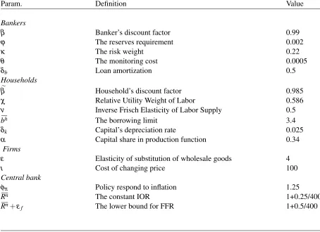
For the bankers’ parameters, we choose the discount factorβ =0.99 to match with the federal

funds rate of 4% annually before the Great Recession. The reserves requirement is set as the

ratio between reserves and the total ZMDs (including checking account, saving account and

money market deposit account) before the financial crisis, which is around ϕ =0.002. The

monitoring costθ and loan amortization δb are set exogenously. The risk weightκ is

exoge-nously set so that 10 percent increase ofκ from steady state will make the capital constraint

binding. (Table6)

Most of the households’ parameters are standard in the literature. The only one that needs

to be calibrated is the borrowing limitbh_{. We calibrate it to match with the ratio between total}

Table 6: Parameter values

Param. Definition Value

Bankers

β Banker’s discount factor 0.99

ϕ The reserves requirement 0.002

κ The risk weight 0.22

θ The monitoring cost 0.0005

δb Loan amortization 0.5

Households

e

β Household’s discount factor 0.985

χ Relative Utility Weight of Labor 0.586

ν Inverse Frisch Elasticity of Labor Supply 0.5

bh _{The borrowing limit 3.4}

δk Capital’s depreciation rate 0.025

α Capital share in production function 0.34

Firms

ε Elasticity of substitution of wholesale goods 4

ι Cost of changing price 100

Central bank

φπ Policy respond to inflation 1.25

Rn _{The constant IOR 1+0.25/400}

Rn_+ε

f The lower bound for FFR 1+0.5/400

other parameters are also in the range which is often seen in the macro literature. We tried using

as few parameters as possible to illustrate the main mechanism of the model.

6.2

Federal funds rate shock

We examine an interest rate shock in the Taylor rule and compare the mechanism of this model

to the standard one in the New Keynesian literature.

R_tf =max

1

β

_πt+1

π

φπ

exp(utf), Rn+εf

R_tn=Rn

u_tf =ρfu_t−f 1, u

f

0 is given

From the steady state, there is an unexpected shock att=0 withu₀f =−2/400, then agents

know that the shock will die slowly withρf =0.6.

Similar to the standard New Keynesian model: As the price is sticky, when the central bank

cut the federal funds rate, the real rate goes down and stimulates the economy in the short run.

(Figure2)9.

Difference from the standard New Keynesian model:

i Banks play an important role in creating money. After the interest rate shock, the real money

balance increases by 0.45 percent. Most of that new money is created by banks when they

increase loans. The amount of money that the central bank actually “drops” to the economy

ˆ

τ to change the federal funds rate only accounts for 0.02 percent of this increase. So unlike

the standard model in New Keynesian, our model focuses on the money creation process by

commercial banks and the pass-through effect from the federal funds rate to the loan rate.

ii Without any adjustment cost functions, investment still well-behaves after the cut in the real

interest rate. The constraint for a huge sudden jump of investment comes naturally from the

ZMD-in-advance constraint and the borrowing constraint.

6.3

Financial Crisis - Taylor Rule Response

From the steady state, we illustrate a financial crisis by imposing an unexpected shock atκt in

the capital constraint. This is a simplified way to reflect a sudden increase in the “potential” bad

loans in the bankers’ balance sheets. This paper does not try answering the cause of the Great

Recession, so this reduced form is neat to assess different monetary policy rules. In this section,

the conventional monetary policy still follows the Taylor rule in (31) and (32).

R_tf =max

1

β

_πt+

1

π

φπ

, Rn_+ε

f

Rn_t =Rn

κt=ρκκt−1+ (1−ρκ)κ, κ0is given

(P2)

9_{Except the federal funds rate and the real borrowing rate are converted to the annual level, all other figures}

0 5 10 15 20 25 30 0 0.5 1 1.5 2 2.5 3 3.5 4 4.5 5 Rf rh Rn

(a) Federal funds rate and real borrowing rate

0 5 10 15 20 25 30

−0.1 0 0.1 0.2 0.3 0.4 0.5 0.6 m

(b) Real balance of ZMDs and Reserves

0 5 10 15 20 25 30

−0.2 0 0.2 0.4 0.6 0.8 1 1.2

1.4 c- B a n k e r ˜

c- H o u s e h o l d s

(c) Consumptions

0 5 10 15 20 25 30

−0.5 0 0.5 1 1.5 2 2.5 3 i k

(d) Investment and Capital

0 5 10 15 20 25 30

−0.02 −0.01 0 0.01 0.02 0.03 0.04 0.05 0.06 0.07 π (e) Inflation

0 5 10 15 20 25 30

−0.1 0 0.1 0.2 0.3 0.4 0.5 0.6

O u t p u t sy

(f) Output

whereρk=0.95 is the persistence of the shock andκ0=0.26, which is 18 percent higher than

the one in the steady state level. The capital requirement switches to the binding mode in the

short run. The response of the economy is illustrated in the Figure3.

The banking crisis is dangerous as it raises the spread between the prime rate and the federal

funds rate. To satisfy the capital requirement (CR), bankers have to cut loans. Loan rate goes

up even when the federal funds rate is cut down, as the shadow price of capital requirementµc t

is positive now.

γt=

β(δb+δbqt+L 1)

πt+1(qtL+θ)

γt+1+

(1−κt)µc

t

q_tL+θ

| {z }

Spread due to CR’s binding

Money supply eventually drops due to the consequence of the debt deleveraging process.

Deflation will be persistent under the Taylor rule as the conventional monetary policy only

focuses on the pass through of federal funds rate to the prime rate, which will not work in this

case.

Standard New Keynesian model emphasizes the importance of monetary policy in correcting

the deviation of real rate from its natural level due the the price stickiness. Under the framework

where the banking sector is modeled clearly, there are two other inefficiencies that monetary

policy can intervene to improve the social welfare. The first inefficiency arises from the binding

of the capital constraints, which freezes the credit market between bankers and households. The

second inefficiency comes from the households’ borrowing constraint itself. Unconventional

monetary policy focuses on the money supply and asset price might be a good remedy for this

situation. We only focus on the money supply in this paper.

6.4

Financial Crisis - Large Scale Asset Purchase (LSAP)

Now, assume that central bank injects money directly into the market by purchasing the

whole-sale firms’ shares. Letxt be the number of shares that central bank decides to hold at timet and

0 10 20 30 40 50 60 70 80 90 100 0 1 2 3 4 5 6 7 Rf rh Rn

(a) Federal funds rate and real borrowing rate

−2 0 2 4 6 8 10

−9 −8 −7 −6 −5 −4 −3 −2 −1 0 1 m bh

(b) Real balance of ZMDs and households’ debts

0 10 20 30 40 50 60 70 80 90 100 −1.4 −1.2 −1 −0.8 −0.6 −0.4 −0.2 0 0.2

(c) Aggregate consumption

−2 0 2 4 6 8 10

−50 −45 −40 −35 −30 −25 −20 −15 −10 −5 0 5 Investment Labor

(d) Investment and Labor

0 50 100 150 200 250 300

−1.2 −1 −0.8 −0.6 −0.4 −0.2 0 0.2 π (e) Inflation

0 20 40 60 80 100 120 140 160 180 200

−8 −7 −6 −5 −4 −3 −2 −1 0 1 2 y (f) Outputs

υtbe the share’s price andxt_e is the number of shares that households hold.

xt+ext =1 (35)

When the central bank makes transactions with households, in the electronic system, the flows

of money will follow the Table7.

The Fed Bankers Households

Securities: +υt∆xt Reserves: +υt∆xt Reserves:+υt∆xt Deposits: +υt∆xt Deposits: +υt∆xt

Securities: -υt∆xt

Table 7: Central Bank’s Asset Purchase

Before time 0, xt =0. At time 0, there is an unexpected shock of purchasing assets from

the central bank in response instantly to the unexpected shock onκ. Then the central bank will

slowly sell these assets back to the market. For the dividends earned from holding securities, we

assume that the consolidated government will give them back to households under the form of

lump-sum transfers. In equilibrium, the equations for reserve flows and deposit flows become:

nt−1

πt

+υt(xt−xt−1) +τˆt=nt (36)

mt=

Rm_t−1mt−1

πt

+qL_tst+θtbht −δb

bh_t−1 πt

+ct+υt(xt−xt−1) +τtˆ −(Rnt−1−1)

nt−1

πt

(37)

The exogenous shock forκt and monetary policy rule are:

κt=ρκκt−1+ (1−ρκ)κ, κ0is given

xt=ρxxt−1, x0is given

ˆ

τt=0, R_tn=Rn_{, ∀t≥0}

(P3)

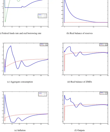
whereρx=0.98 be the persistence of the asset purchasing shock andx0=0.0008. We assume

that the central bank does not follow the Taylor rule anymore. They still fix the interest on

reserves at the constant level Rn and only use that asset purchase/sale program to adjust the

0 50 100 150 200 250 300 −8 −6 −4 −2 0 2 4 6

Rf- L S A P

rh- L S A P

Rn

(a) Federal funds rate and real borrowing rate

0 50 100 150

−100 0 100 200 300 400 500 600 700

n − LSAP n − Taylor

(b) Real balance of reserves

0 50 100 150 200 250 300 −2 −1.5 −1 −0.5 0 0.5 1 1.5 2

C − LSAP C − Taylor

(c) Aggregate consumption

0 50 100 150 200 250 300 −10 −8 −6 −4 −2 0 2 4

m − LSAP m − Taylor

(d) Real balance of ZMDs

0 50 100 150 200 250 300

−1.5 −1 −0.5 0 0.5 1 1.5 2 2.5 3 3.5

π- L S A P

π- Tay l o r

(e) Inflation

0 50 100 150 200 250 300

−8 −6 −4 −2 0 2 4 6

y − LSAP y − Taylor

(f) Outputs

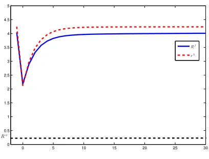
Here are some important remark for LSAP’s effect:

i The excess reserves skyrockets and the long duration of the federal funds rate at the lower

bound: When the central bank purchases assets from the private sector, they inject

simul-taneously the money supply into the market and banking reserves into the banking system.

When the level of reserves increases by 700 percent, the reserve constraint is no longer

binding, µr

t =0. As we assume that the central bank fixes IOR at a constant level, it is

synonymous that the federal funds rate will be at the lower bound for a long time, around

25 years (100 quarters) in our model. After a long unwinding quantitative easing process,

the reserve requirement will be binding again. The federal funds rate climbs back to its long

run level. The whole transition process can take around 80 years in our model.

ii Positive effect in the short-run: The combination of new money injection and the long

dura-tion of the federal funds rate at the lower bound steer the economy out of recession quickly,

unlike the case with the Taylor rule. As loans have the longer maturity than deposits, if the

central bank commits to let the federal funds rate at the low level for a long time, the real

lending rate will decline sharply. It combines with the relaxation of the liquidity constraint,

stimulating the household’s demand and pushing up inflation.

iii Negative effect in the long-run: After inflation jumps up in the short run, it starts declining,

below the central bank’s target. This phenomenon can be explained by the Neo-Fisherian’s

idea. In the long run, real short-term rate will be back to the long-term level. AsR_tf =Rn,

the deflation must realize to increaseR_tf/πt+1.

iv Intuitive Explanation: When the central bank keeps the interbank rate at 25 basis points, the

rate of saving account Rm will be at 25 basis points as deposits and interbank loans have

the same short-term maturity. However, the real return on capital in the long-run recovers

to the pre-crisis level. In equilibrium, the real return on money (plus the liquidity premium)

must follow the real return on capital. The endogenous money supply declines gradually.

6.5

Interest on Reserves (IOR) as Monetary Policy Tool

6.5.1 IOR: To raise or not to raise?

In the previous section, we know that after the LSAP program without adjustingR_tn, the inflation

- the central bank’s main target - is high in the short run but below the target in the long-run.

How long should the central bank keep the federal funds rate at the zero lower bound? And if

the central bank decides to raise rate, what is the best strategy for the central bank?

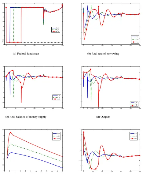
In this section, we still conduct the experiment similar to the previous section with one twist.

We assume that afterTuperiods, the central bank will raise IOR and afterTd periods, IOR will

be brought back to the initial level. We choose the different level forTuat 20, 40 and 80 quarters

to see the effect of the prolonged low interest rate environment on output and inflation in the

short run and long run.Tdis chosen at 200 quarters.

κt=ρκκt−1+ (1−ρκ)κ, κ0is given

xt=ρxxt−1, x0is given

ˆ

τt=0, ∀t≥0

Rn_t =

      

     

Rn _ift<Tu

1/β ifTu≤t≤Td

Rn _ift>T

d

(P4)

Here are some remarks from our experiments: (Figure5)

i. The longer is the duration of the federal funds rate at the lower bound, the higher is inflation

in the short run. This forward guidance effect is well-documented in the New Keynesian

literature when the central bank commits to set the short-term at the zero lower bound for a

long time (Eggertsson and Woodford(2003) ). However, the hyperinflation never happens in our model even with 20 years that rate is set at the lower bound. Due to the household’s

borrowing constraint and banker’s capital constraint, the amount of the money supply is

0 50 100 150 200 250 300 0 0.5 1 1.5 2 2.5 3 3.5 4 4.5 Rf_20 Rf_40 Rf_80 Rn

(a) Federal funds rate

0 50 100 150 200 250 300

−6 −4 −2 0 2 4 6 8

rh2 0

rh4 0

rh8 0

(b) Real rate of borrowing

0 50 100 150 200 250 300

−12 −10 −8 −6 −4 −2 0 2 4 m_20 m_40 m_80

(c) Real balance of money supply

0 20 40 50 80 100 150 200 250 300

−10 −8 −6 −4 −2 0 2 4 y_20 y_40 y_80 (d) Outputs

−2 0 2 4 6 8 10 12 14 16 18 20

−1 −0.5 0 0.5 1 1.5 2 2.5

π2 0

π4 0

π8 0

(e) Inflation - Short run

0 50 100 150 200 250 300 −1.5 −1 −0.5 0 0.5 1 1.5 2 2.5

π2 0

π4 0

π8 0

(f) Inflation - Long run

ii. The longer is the duration of the federal funds rate at the lower bound, the bigger is the

negative effect on output and deflation in the long run. It emphasizes that our model is

Keynesian in the short run, but Neo-Fisherian in the long run.

iii. The endogenous money supply drops sharply when the central bank raises rates. As price

is sticky, the real fed funds rate and real lending rate must go up after this rate hike. Hence,

the total of amount of bank credits declines, also implying a huge fall in the money supply.

However, after some periods, the neo-Fisherian effect dominates the Keynesian effect,

sta-bilizing inflation at the target level. After all, the central bank still needs to pay a big cost

for a rate hike in the short run.

The last point implies an important hint for monetary policy when the central bank decides to

raise rate. The central bank can still stabilize inflation and the aggregate demand if it commits

to a rule of targeting the money supply at the time of raising rates. The appearance of interest

on reserves and electronic payment system allow the central bank to manipulate both the money

supply and interest rate at the short run, which is very different from Keynesian theory with only

paper money. In this sense, our research is very near to the Monetarism when the growth rate of

the money supply always decides the inflation path in the long run.

6.5.2 Raise rate and raise money supply - Money Supply Rule

We do an experiment similar to (P4) but at the time of raising IOR, the central bank also commits

to a money supply rule (massive helicopter money if necessary) to target the inflation rate. The

money supply rule simply responds to the deviation of the inflation rate from its target:

Mt

Mt−1

=

π πt

ρm

(38)

whereρm=0.5 is the coefficient showing how much the central bank will change the growth

rate of the money supply in response to inflation.

To create the same interest path like the previous section, we assume this money supply

exogenous shocks and monetary policy for this experiment can be written as follows:

κt =ρκκt−1+ (1−ρκ)κ, κ0is given

xt =ρxxt−1, x0is given

      

ˆ

τt=0 ift<Tu

log(mt)−log(mt−1) =−(1+ρm)log(πt) ift≥Tu

R_tn=

            

Rn _ift<Tu

1/β ifTu≤t≤Td

Rn _ift>T

d

(P5)

Figure6, by comparing (P5) to (P4), shows the effectiveness of combining raise rate with the rule of targeting money supply:

i. Even though the federal funds rate paths are nearly identical in the first 200 periods in our

experiments, the dynamics of output and inflation are very different. It implies that interest

rate path does not give enough information for the stance of monetary policy when central

bank use IOR as the main tool. When there is no excess reserves, federal funds rate path

conveys all information about monetary policy. It is not this case with the current situation,

when the central bank can manipulate both money supply and interest rate.

ii. Money supply targeting is extremely efficient in stabilizing inflation and output. The

infla-tion is anchored at the target rate since the time the central bank target the growth rate of

the money supply in our model.

iii. At the time of raising rate (period 20), to stabilize the inflation and avoid a severe short

recession, money supply targeting implies that the central bank should conduct a massive

helicopter money. With this commitment, the central bank can anchor the household’s

0 50 100 150 200 250 300 0 0.5 1 1.5 2 2.5 3 3.5 4 4.5

Rf- M S R u l e Rf- L S A P 2 0

¯

Rn

(a) Federal funds rate

0 50 100 150 200 250 300

−8 −7 −6 −5 −4 −3 −2 −1 0 1 2

m- M S r u l e

m- L S A P 2 0

(b) Real balance of ZMDs

15 16 17 18 19 20 21 22 23 24 25

−0.01 −0.005 0 0.005 0.01 0.015 0.02

τ- M S r u l e

τ- L S A P 2 0

(c) The amount of money drops (level)

0 50 100 150 200 250 300 −1 −0.5 0 0.5 1 1.5 2 2.5

π- M S r u l e

π- L S A P 2 0

(d) Inflation

0 5 10 15 20 25 30 35 40 45 50 −7 −6 −5 −4 −3 −2 −1 0 1 2 3

y- M S r u l e

y- L S A P 2 0

(e) Output - Short run

0 50 100 150 200 250 300

−7 −6 −5 −4 −3 −2 −1 0 1 2 3

y- M S r u l e y- L S A P 2 0

(f) Output - Long run

7

Conclusion

Our research shows that, when the central bank controls the federal funds rate by adjusting

interest on reserves, the interest path does not provide full information on the stance of monetary

policy. The endogenous money supply can complete go down when the federal funds rate is near

zero for a long time. However, if the central bank simply raises rate, the economy will fall into

a short recession and deflation is worse in the short run. Basically, the central bank falls into a

dilemma to raise or not to raise rate, where outcome is not bright in either way.

One feasible solution for the central bank is to target the growth rate of the money supply

in response to inflation when they raise rates. With that, they can completely avoid the negative

References

Abel, Andrew B. 1985. “Dynamic Behavior of Capital Accumulation in a Cash-in-Advance Model.” National Bureau of Economic Research, Inc NBER Working Papers 1549.

Afonso, Gara, and Ricardo Lagos.2015. “Trade Dynamics in the Market for Federal Funds.”

Econometrica, 83: 263–313.

Becker, William E.1975. “Determinants of the United States Currency-Demand Deposit Ra-tio.”The Journal of Finance, 30(1): 57–74.

Belongia, Michael T., and Peter N. Ireland.2006. “The Own-Price of Money and the Channels of Monetary Transmission.”Journal of Money, Credit and Banking, 38(2): 429–445.

Belongia, Michael T., and Peter N. Ireland.2014. “The Barnett critique after three decades: A New Keynesian analysis.”Journal of Econometrics, 183(1): 5–21.

Bernanke, Ben S., Mark Gertler, and Simon Gilchrist.1999. “The financial accelerator in a quantitative business cycle framework.” In Handbook of Macroeconomics. Vol. 1 of

Hand-book of Macroeconomics, , ed. J. B. Taylor and M. Woodford, Chapter 21, 1341–1393.

Else-vier.

Bianchi, Javier, and Saki Bigio.2014. “Banks, Liquidity Management and Monetary Policy.” National Bureau of Economic Research, Inc NBER Working Papers 20490.

Brunnermeier, Markus, and Yuliy Sannikov.2016. “The I Theory of Money.” National Bu-reau of Economic Research, Inc NBER Working Papers 22533.

Christiano, Lawrence J., Roberto Motto, and Massimo Rostagno.2004. “The Great Depres-sion and the Friedman-Schwartz hypothesis.” Federal Reserve Bank of Cleveland Working Paper 0318.

Cochrane, John H. 2014. “Monetary policy with interest on reserves.” Journal of Economic

Dynamics and Control, 49: 74–108.

Cochrane, John H.2016. “Do higher interest rates raise or lower inflation?” Unpublished

pa-per, February, https://faculty. chicagobooth. edu/john. cochrane/research/papers/fisher. pdf.

Curdia, Vasco, and Michael Woodford.2011. “The central-bank balance sheet as an instru-ment of monetarypolicy.”Journal of Monetary Economics, 58(1): 54–79.

Dotsey, Michael.1983. “An examination of implicit interest rates on demand deposits.”

Eco-nomic Review, , (Sep): 3–11.

Eggertsson, Gauti B., and Michael Woodford.2003. “The Zero Bound on Interest Rates and Optimal Monetary Policy.”Brookings Papers on Economic Activity, 34(1): 139–235.

Friedman, Milton.1959. “The Demand for Money: Some Theoretical and Empirical Results.”

Fuerst, Timothy S.1992. “Liquidity, loanable funds, and real activity.” Journal of Monetary

Economics, 29(1): 3–24.

Gertler, Mark, and Nobuhiro Kiyotaki. 2010. “Financial Intermediation and Credit Policy in Business Cycle Analysis.” InHandbook of Monetary Economics. Vol. 3. 1 ed., , ed. Ben-jamin M. Friedman and Michael Woodford, Chapter 11, 547–599. Elsevier.

Gertler, Mark, and Peter Karadi.2011. “A model of unconventional monetary policy.”

Jour-nal of Monetary Economics, 58(1): 17–34.

Goodfriend, Marvin, et al.2002. “Interest on reserves and monetary policy.”Federal Reserve

Bank of New York Economic Policy Review, 8(1): 77–84.

Iacoviello, Matteo.2005. “House Prices, Borrowing Constraints, and Monetary Policy in the Business Cycle.”American Economic Review, 95(3): 739–764.

Ireland, Peter N.2014. “The macroeconomic effects of interest on reserves.”Macroeconomic

Dynamics, 18(6): 1271–1312.

Judson, Ruth.2012. “Crisis and calm: Demand for U.S. currency at home and abroad from the fall of the Berlin Wall to 2011.” Board of Governors of the Federal Reserve System (U.S.) International Finance Discussion Papers 1058.

Keister, Todd.2016. “Interest on Reserves.” InTestimony before the Subcommittee on Monetary

Policy and Trade. Committe of Financial Services, United States House of Representatives,

May 17.

Keister, Todd, and James McAndrews. 2009. “Why are banks holding so many excess re-serves?”

Kiyotaki, Nobuhiro, and John Moore.1997. “Credit Cycles.”Journal of Political Economy, 105(2): 211–48.

Leland, Hayne, and Klaus Bjerre Toft. 1996. “Optimal Capital Structure, Endogenous Bankruptcy, and the Term Structure of Credit Spreads.”Journal of Finance, 51(3): 987–1019.

Lucas, Robert E, Jr, and Nancy L Stokey.1987. “Money and Interest in a Cash-in-Advance Economy.”Econometrica, 55(3): 491–513.

McGrattan, Ellen R. 1996. “Solving the stochastic growth model with a finite element method.”Journal of Economic Dynamics and Control, 20(1-3): 19–42.

Mishkin, Frederic S.2007.The economics of money, banking, and financial markets.Pearson education.

Mitchell, Douglas W. 1979. “Explicit and Implicit Demand Deposit Interest: Substitutes or Complements from the Bank’s Point of View?” Journal of Money, Credit and Banking, 11(2): 182–191.

Ngotran, Duong. 2016. “The E-Monetary Theory.” University Library of Munich, Germany MPRA Paper 77206.

Sargent, Thomas, and Neil Wallace.1985. “Interest on reserves.”Journal of Monetary

Eco-nomics, 15(3): 279–290.

Schmedders, Karl, Kenneth L Judd, and Felix Kubler.2002. “A solution method for incom-plete asset markets wih heterogeneous agents.”

Sheard, Paul.2013. “Repeat after Me: Banks Cannot and Do Not Lend Out Reserves.”Credit Market Services, Standard and Poor´s, available at http://issuu.

com/positivemoney/docs/sp-banks-cannot-anddo-notlend-out.

Startz, Richard.1979. “Implicit interest on demand deposits.”Journal of Monetary Economics, 5(4): 515–534.

Stockman, Alan C. 1981. “Anticipated inflation and the capital stock in a cash in-advance economy.”Journal of Monetary Economics, 8(3): 387–393.

Wachter, Andreas, and T. Lorenz Biegler.2006. “On the implementation of an interior-point filter line-search algorithm for large-scale nonlinear programming.”Mathematical Program-ming, 106(1): 25–57.

Wang, Peng-fei, and Yi Wen. 2006. “Another look at sticky prices and output persistence.”

Journal of Economic Dynamics and Control, 30(12): 2533–2552.

Zangwill, Willard I, and CB Garcia.1981.Pathways to solutions, fixed points, and equilibria.

A

Mathematical Appendix

Proof for Theorem1:

From the first order condition of bankers’ problem, we have:

γt = βR

f

tγt+1

πt+1

+µ_tc (A.1)

γt =

βR_tmγt+1

πt+1

+µ_tc+ϕ µ_tr (A.2)

γt =

βR_tnγt+1

πt+1

+µ_tc+µ_tr (A.3)

Asµc

t andµtrare non-negative shadow price of capital constraint and reserve constraint, γt>0

asct>0, we haveRnt ≤Rmt ≤R f t.

The′′=′′ happens whenµ_tr =0, or when the reserver requirement is no longer binding.

Proof for Theorem2:

The equation for reserves flow (1) is:

R_t−n ₁n_t−1

πt

+R

f

t−1b

f

t−1

πt

+dt+et+τt=nt+btf

In equilibrium,b_tf =0,dt+et =0 and from (30):

τt=−

(Rn

t−1−1)nt−1

πt

+τˆt

Substitute that into the reserves flow:

nt−1

πt

+τˆt=nt

So the total level of reserves only depend on ˆτ, which is decided solely be the central bank.

Proof for Theorem3:

state:

π= 1

1−τ/n (A.4)

Under the Assumption (2):

τ

n =

π−1

π (A.5)

(A.4) and (A.5) →π=π. Money supply rule ensures that inflation reaches to its target in the steady state.

From (32), we have:

Rf =max{π/β,Rn_+ε

f} (A.6)

Under the assumption (2): Rn_+ε

f <π/β, we get Rf =π/β. The equation (A.1) can be

rewritten in the steady state as:

γ = βR

f_γ

π +µ

c

WhenRf =π/β, we getµc=0, the capital constraint is not binding (if steady state exists). As

Rf >Rn_{, from the Theorem1, µ}r _{>0, or the reserve requirement is binding.}

Whenµc_{=0, from (10), at the steady state:}

qL =β δb−θ π

π−β δb

(A.7)

Under the Assump