Evolution in a Walrasian setting

Munich Personal RePEc Archive

Evolution in a Walrasian setting

Accinelli, Elvio and Covarrubias, Enrique

June 2015

Online at

https://mpra.ub.uni-muenchen.de/64736/

Evolution in a Walrasian setting

∗

E. Accinelli

E. Covarrubias

Abstract

This paper models the dynamic of a sector where firms imitate the technology of leading firms. While it would seem natural to expect that managers will aim at producing with the technology that produces the highest benefits, if many other managers also follow this behavior, the market structure might be modified so much that the advantage associated with a high-profit technology might be erased or even reverse. By modeling this imitation process with replicating dynamics, we find that even if the parameters of the economy are continuous through time and the economy follows a path of competitive equilibria, endogenous discrete jumps in technological choices occur.

∗_{The authors thank Mario Ibarburu and participants of seminars at the Economics}

Department of the Social Sciences School, Uruguay, for useful comments.

†_{Facultad de Econom´ıa, Universidad Aut´onoma de San Luis Potos´ı. M´exico. E-mail:}

[email protected]

‡_{Banco de M´exico, Av. 5 de mayo 18, Col. Centro, Mexico City. E-mail:}

[email protected]

1 Introduction 2

1

Introduction

Managers of firms are confronted continuously with the decision of whether to keep producing with their firm’s existing technology or to shift to other leading alternatives. It would seem natural for a manager, even under in-complete information, to observe available technologies and to choose for his firm the one that gives rise to the highest profits to other firms that already have it. However, some markets might provide a certain advantage if not too many producers are using the same technology so that, if too many man-agers choose it simultaneously, the benefits of this technology might even be reversed. In other words, if a manager decides to switch to a technology that is observed to have the highest profits, it could be the case that many other managers also make the same decision simultaneously.

This paper has two main contributions. On the hand, it proposes a the-oretical model to study this dynamic game of imitation under incomplete information. To do so, we propose an approach using replicating dynamics, extending this way the work of Schlag (1998), Harrington et al. (2005), Ania (2008), Bergin and Bernhardt (2009), Apesteguia et al. (2010) and Duersch et al. (2012). On the other hand, and more importantly, we characterize dynamics along its equilibrium path and find that, under robust conditions, even being always in equilibrium, endogenous jumps in equilibrium variables can occur.1 _{As in (Perla and Tonetti, 2014) we consider a distribution of}

het-erogeneous firms producing with hethet-erogeneous technologies, but we consider the rates of profits as the real engine of the decisions of managers. Indeed, we do not focus on growth, but instead our main point of attention is on the characteristic of the equilibrium manifold and the evolution along an equi-librium path on this manifold, showing that “technological crises” can occur as a result of rational decisions.

This paper is structured as follows. Section 2 presents the model of a private-ownership economy, its parameters, and the definition of equilibrium. In particular, we will define firms, consumers and Walrasian equilibria. Sec-tion 3 defines the equilibrium set and studies its properties. To do so, we study excess demand functions, as well as regular and critical economies.

1

2 The economy 3

The dynamical behaviour of pure system is introduced in section 4. We con-sider that imitation play a significant role when the decision makers have incomplete information. In section 5 we analyze the stability of the dy-namical equilibrium using the Liapunov method. In section 6 we consider a numerical example and finally, some conclusions are given.

2

The economy

In this section, we introduce the model of our economy. We will consider a competitive market with two goods, two types of firms and two types of consumers. Within each type, firms will use identical technologies, while consumers will have identical preferences, and endowments of both goods and shares in companies. We will assume that markets are competitive in the sense that every good is traded in the market at a publicly known price, and consumers trade to maximize their own welfare, while firms produce to maximize profits. We will formalize the structure of consumers, firms and equilibria in this section.

Since there are two goods in the economy, thecommodity spaceisR2while the consumption set and price set is R2+ ={x = (x1, x2)∈ R2 : x1, x2 ≥0}.

We will also use the notation R2++={x= (x1, x2)∈R2 :x1, x2 >0}.

2.1

Firms

We consider an economy with a finite but large number N of firms, which will be indexed by F = {1, . . . , N}. There will be two types j ∈ {1,2} of such firms. There aren1 firms of type 1 and n2 of type 2, withn1+n2 =N.

We will index firms within each type by Fj = {0, ..., nj}, with at least one

firm of one of the two types. The proportion of firms of type j is given by

Nj =nj/N, and one should keep in mind that as N → ∞, Nj takes values in the continuum [0,1].

Firms are characterized by their technological set Y1 or Y2, according to

2 The economy 4

of profit. The set of available technologies will be denoted by T ={Y1, Y2}.

We consider that there is no principal-agent problem, that is, that the inter-ests of managers are the same of owners, which is to maximize profits. We assume that technological sets satisfy the following standard properties, for

j ={1,2}: (i) Yj is closed and convex; (ii) Yj ∩R2+ = {0}; (iii) −R2+ ⊂Yj;

and, (iv) Yj is bounded from above, i.e., there exists someaj ∈R2+ satisfying

y≤aj for all y∈Yj.2

If Yj is a production set and p ∈ R2++ is a price vector, then the profit

function at price level pis the function πj _{:Yj →R defined byπ}j_{(y) =p·y.}

Thus, firm j ’s goal is to solve the problem

max

y∈Yj

p·y, (1)

The function yj _:

R2++ → R2 that solves problem (1) is the supply of a

firm of type j ∈ {1,2}. When summarising the supply functions of all firms in the economy we will use the notation y = (y1_,y2_{) ∈ R}2n1 ×_R2n2, where

yj _{is the vector of supply functions of thenj firms of type j.}

2.2

Consumers

The are M consumers in the economy distributed into type 1 or type 2. We will index consumers by I = {1, . . . , M}. There are mi consumers of type i, i ∈ {1,2}, with m1 +m2 = M. Therefore, the proportion of

con-sumers of type i is Mi = mi/M. We will index consumers in each type by

Ii = {0, . . . , mi} with at least one consumer of one type. All consumers of type i have identical C∞ _{utilities ui :}

R2+ → R and identical initial

endow-ments of goodswi _{= (w}i

1, wi2)∈R2+. We assume utilities satisfy the following

standard properties: (i) the bordered Hessian of ui is non-zero at every x; (ii) the set {x′ _:u(x′_{)≥u(x)}is closed in}

R2 for every x∈_R2 ++.3

The wealth of a consumers is derived from individual endowments of commodities but also from ownership claims (shares) of profits of firms, which

2

As is standard, it is sometimes convenient to describe the production set using a function Fj : R2 → R such that Yj ⊂ R2 and Fj(x1, x2) ≤ 0, ∀(x1, x2) ∈ Yj, and

F(x1, x2) = 0 if and only if (x1, x2) is an element of the boundary ofYj.These functions

are called technological functions. See for instance (Mas-Colell, 1989).

3

2 The economy 5

we also assume to be identical within types. Hence, each consumeri∈I has a claim to a non-negative share θij of the profit of each firm j ∈ F in a way that PM

i=1θij = 1 for eachj. This implies that the individual wealthWi of a

consumer of type i is given by

Wi_(n

1, n2, p) = p·wi+n1θi1π1(p) +n2θi2π2(p).

It is important to highlight that the wealth of an individual depends on the distribution (n1, n2) of firms in the economy. In the next section, when

we introduce dynamics to our model, this distribution will change endoge-nously so that the actions of a manager looking to use the most profitable technologies will have an immediate impact over the wealth of agents.

Now, the budget set Bi _{of a consumer of type i is given by} Bi_(n

1, n2, p) = {xi ∈R2+:p·xi ≤Wi(n1, n2, p)}.

Thus, given the distribution of firms (n1, n2) and price level p, the

opti-mization problem of a consumer of type i is given by max

x∈_R2₊

ui(x) s.t. x ∈Bi(n1, n2, p). (2)

The functionxi _:

R2++ →R2that solves optimization problem (2) is called

the individual demand function of a consumer of type i. When summarising the demand functions of all consumers in the economy, we will use the nota-tion x= (x1_,x2_)∈R2m1×_R2m2, where xi is the vector of demand functions

of the mi consumers of typei.

2.3

Walrasian equilibrium

As discussed above, a private-ownership economy is determined by the fol-lowing factors: the number and distribution of firms (n1, n2) and their

tech-nologies (Y1, Y2); the number and distribution of consumers (m1, m2), their

preferences (u1, u2), their initial endowments (w1, w2), and their portfolios of

shares (θ11, θ12, θ21, θ22). This gives rise to the following definition.

Definition 1 (Private-ownership economies): A private ownership economy E

is a choice of parameters (nj, Yj, mi, ui, wi, θij) with i, j = {1,2}. We will write

3 The equilibrium set 6

Now, the notion of a price-taking equilibrium for a competitive private ownership economy is that of a Walrasian equilibrium, which we now define.

Definition 2 (Walarsian equilibrium): Consider a private-ownership economy

E(nj, Yj, mi, ui, wi, θij).

We say that a vector of demand-supply functions (x∗

,y∗

) = (x1∗

,x2∗

,y1∗

,y2∗

) and a system of prices p∗

= (p∗ 1, p

∗

2) constitute a Walrasian equilibrium, or

competitive equilibrium, if:

1. For each firm inF, yj∗

solves the optimisation problem (1) of a firm of type j;.

2. For each agent in I, xi∗

solves the optimisation problem (2) of a con-sumer of type i;.

3. Aggregate demand equals aggregate supply. That is,

m1

X

i=1

x1∗

i + m2

X

i=1

x2∗

i =m1w1+m2w2+

n1

X

j=1

y1∗

j + n2

X

j=1

y2∗

j .

Note in Definiton (2), that the market-clearing condition can be written succinctly as

m1 x1∗−w1+m2 x2∗−w2 =n1y1∗+n2y2∗. (3)

3

The equilibrium set

Through the rest of the paper, we will suppose (Yj, mi, ui, wi, θij) are all fixed parameters. That is, we will suppose that the only parameter of the econ-omy is the distribution of firms (n1, n2) according to its type. Furthermore,

we will also suppose that the total number of firms N is fixed (albeit very large). With this assumption, n2 is determined once a choice of n1 is made

since n2 =N−n1. To highlight this choice of parameters, we will denote an

economy by E(N,Yj,mi,ui,wi,θij)(n1) or, if no confusion arises, simply by E(n1).

3 The equilibrium set 7

n1.

In this section we will explore the equilibrium set of an economy E(n1).

Recall that the Walrasian corresponde is the set-valued function that assigns to each economy E(n1) its set of competitive equilibria. This idea gives rise

to the notion of theequilibrium set as the set of all pairseconomies-equilibria. We will show that studying this set is an important first step in our analysis. Thus, in this section we formalize the notion of excess demand functions, the equilibrium set and regular and critical economies. Intuitively, a regu-lar economy n1 is one where equilibrium prices will be determinate (that is,

prices are locally continuous functions of n1, while a critical economy is one

where small perturbations ofn1 lead to large perturbations of its equilibirum

price.

3.1

Excess demand functions

The notion of a competitive equilibrium can be rephrased in terms of zeroes of aggregate excess demand functions. To see this, consider the private-ownership economy E(n1). For a fixed n1, we say that the individual excess

demand function ζi n1 :R

2

++→R2 of a consumer of type i is given by

ζi

n1(p) = x

i

n1(p)−w

i_.

Similarly, for a fixed economy n1 we define the aggregate excess demand

function of this economy, Ψn1 = (Ψ

1

n1,Ψ

2

n1) :R

2

++ →R2, by

Ψn1(p) =m1ζ

1

n1(p) +m2ζ

2

n2(p)−n1y

1_(p)−n

2y2(p).

Notice that the aggregate excess demand function Ψn1 of economy E(n1)

satisfies the following properties:

• Ψn1 is homogeneous of degree zero, i.e., Ψn1(λp) = Ψn1(p) for allλ >0;

• Ψn1 satisfies Walras law, i.e., p·Ψn1(p) = 0, for all p.

3.2

The equilibrium set

3 The equilibrium set 8

Ψn1(p) = 0. We denote the equilibrium set of economy E(n1) by

Γn1 ={p∈R

2

++: Ψn1(p) = 0} ⊂R

2 ++.

Notice that for each equilibrium price, demand and supply functions (x,y) are fully determined so equilibrium prices also determine fully Wal-rasian equilibria. Whenever it is convenient to highlight that the parameter

n1 is changing, we will explicitly write this dependence in the excess demand

function by Ψn1(p) = Ψ(n1, p) and its corresponding equilibrium set by

Γ ={(n1, p) : Ψ(n1, p) = 0}.

Since excess demand functions satisfy homogeneity of degree zero, it al-lows us to choose a suitable price normalization; thus, we will let prices to be in the simplex

∆ =

(p1, p2)∈R+2 :p1+p2 = 1 .

Note that, if p is in the simplex and p2 is known, then p1 is also known,

sincep1 = 1−p2. Also notice that, from Walras law,p1Ψ1n1(p)+p2Ψ

2

n1(p) = 0

for all p. Combined, these two facts suggest we can consider a restricted excess demand function Ψˆn1 : [0,1]→Rsuch that ˆΨn1(p1) = Ψ

1

n1(p). Hence,

a price p = (p1, p2) is an equilibrium for the economy E(n1) if and only if

ˆ

Ψn1(p1) = 0. Thus the set Γn1 can also be represented as

Γn1 =

n

p∈∆ : ˆΨn1(p1) = 0

o

⊂∆.

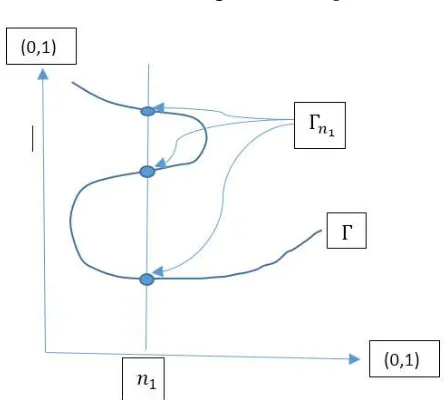
Figure 1 shows the intuition behind the equilibrium sets Γ and Γn1. First,

notice that the horizontal axis consists of the set of economies. Similarly, the vertical axis shows the possible values of prices p which is isomorphic to the set [0,1]. Now, for a fixed economy n1 as depicted, its equilibria (three in

this case) form the set Γn1. All pairs economies-equilibria together form the

set Γ.

3.3

Regular and critical private-ownership economies

The previous figure showed the intuition behind the equilibrium set Γ.4 _If

this diagram were a true representation of our model, one could see that there

4

3 The equilibrium set 9

Fig. 1: The equilibrium set Γ.

are two types of economies. On the one hand, there are economies such as n1

where each price equilibrium has the property that small (i.e. infinitesimal) perturbations to n1 would be accompanied by small changes in this

equilib-rium price. A price with this property will be called a regular price. Notice that, under this intuition, all equilibrium prices of n1 are regular. When this

is the case, the economy (that is, n1) will be called a regular economy.

On the other hand, notice that economy n′

1 has a different structure.

While the lower equilibrium is regular (since an infinitesimal perturbation of n′

1 leads to a small perturbation in this equilibrium price), the upper

equilibrium is different. In this case, a perturbation n′

1 −ǫ of n ′

1 would be

accompanied by a continuous change of the price along one of the branches, but a perturbation n′

1+ǫ ofn ′

1 would lead to ajump of the equilibrium price

4 Dynamical behaviour 10

Definition 3 (Regular and critical prices): Consider a private ownership econ-omy E(n1), with its corresponding excess demand function Ψn1 : ∆ → R

2_,

and equilibrium price set Γn1 ={p∈∆ : Ψn1(p) = 0}. Then, we say that an

equilibrium price p is a regular price if and only if the rank of the Jacobian of the excess demand function evaluated at p is equal to 1. Otherwise, we say pis a critical price.

Definition 4 (Regular and critical economies): We say that an economy E(n1)

is regular if all of its equilibrium prices are regular. If at least one if its equilibrium prices is critical, we say the economy is critical.

As a consequence of the Sard-Smale Theorem it follows that the set of regular economies form an open and dense subset of the set of economies. This means that if a regular economy suffers a perturbation on its funda-mentals the perturbed economy remains regular. This, however, stops being true if the economy is singular. Nevertheless, the set of critical economies is “ meager” in the set of economies, that is, it is a subset of Lebesgue-measure zero.

4

Dynamical behaviour

Suppose that in equilibrium at time t, the distribution of firms is given by

N(t) = (N1(t), N2(t)) and that the share profits of a firm of type Yi are

4 Dynamical behaviour 11

The key question is then based on which factors will managers make the decision of changing technologies used, given that until now they do not know what others are doing. Regardless of the answer to this question, it seems natural to assume that the number of firms producing according to the technology that in each time appears to be the most successful increases. Equivalently, at each time, the share of firms producing according with the technology with the highest profits increases. Such evolutionary process can be modeled by replicating dynamics. In this way, this dynamical behaviour becomes a good tool to describe and understand the evolution of the econ-omy. This section introduces this dynamical behaviour to a private-ownership economy, first as a static game, and then by an evolutionary process.

As in previous Sections, we suppose there is a a finite (albeit very large) number of firms N. We suppose this number remains constant (i.e., no en-tries or exits), although each firm will endogenously change its type through time. At each time period t, the number of firms of type j ∈ {1,2}, is given by nj so that N = n1(t) +n2(t), ∀t. The proportion of firms of type j at

each t is thus given by Nj(t) = nj(t)/N.

4.1

Static game

Consider the private-ownership economy E(n1). The distribution of firms is

thus given by (N1, N2). In this situation, the manager of each company must

choose between changing its existing technology or to keep it. It is possi-ble to model this situation as a N−population normal form game, where each firm has two available strategies T = {Y1, Y2}. Recall that the

sup-ply of a firm of type j ∈ {1,2} is the function yj : R2++ → R2, and its

profit function is given by πj : Yj → _R. The function π∗

i : ∆ → R defined

by π∗

i(N1, N2) = πi(y∗i(N1, N2)) represents the profits in equilibrium of a

firm operating according with the technology Yj. Consequently we will let Π∗

i(N1, N2) = Πi(y∗i(N1, N2)) to symbolize the rate of profits of a firm of

4 Dynamical behaviour 12

Definition 5: We say that to produce according with Yj is a best response given the distributionN = (N1, N2),if the rate of profits producing according

with technology Yj is greater than or equal to the percentage obtained when produced according to the technology Yi. That is,

Πj(y∗j(N))≥Πi(y∗i(N)).

Definition 6: A distributionN∗

= (N∗ 1, N

∗

2) is an equilibrium distribution (or

an equilibrium in mixed strategies) for this game if and only if

Πj(y

∗j_(N∗

)) = Πi(y

∗i_(N∗

)) (4)

for all i, j ∈ {1,2}.

Therefore, a Nash equilibrium for theN −population game

G={Yi, Ni, i∈ {1,2,}}

is a distribution N∗

verifying equation 4.

4.2

Evolution

When introducing time to the static game defined above, dynamic competi-tion increases difficulties for managers. Indeed, they know that from time to time they will have to make sudden decisions even if they do not feel ready to act, because otherwise one or more competitors will come up with a bet-ter solution, pushing a firm to exit. Certainly, if owners lack information or sufficient time to perform calculations, some mistakes in decisions can hap-pen. In this framework to imitate the behavior of the agents considered most successful can be a good strategy. So, a bounded rational vision of the top competent team set the direction of the firm and define the competence of the owner or manager involved. One of the fundamental issue in evolutionary game theory concerns the relationship between predictions as consequence of myopic decisions made by simple agents and those provided by traditional rationality-based concepts.

We start this section by introducing a replicating dynamical system in Definition 7 below. Recall that equilibrium supply functions depend on the distribution of firms so that y∗

i =y

∗

4 Dynamical behaviour 13

4.2.1 The replicator dynamical system

The degree of competition in a given economy depend on the variance on the profit rates, the larger the spread the grater the degree of dynamic competi-tion will be. In equilibrium essentially all the firms are obtaining the same result. I the next definition we introduce a function that measure the degree of dynamical competition in an economy, from the difference in profit rates.

Definition 7: (Augmented replicating dynamical system) Consider an

economy n1 where prices are given by p∗(n1) ∈ Γn1. Let φ : R → R be a

continuous, increasing function such that φ(0) = 0. Then, the (augmented) replicating dynamical system is given by

d dtNi =

φi Πi(y∗i(N))−Πj yj∗(N) Ni, (i)

d

dtNj =− d

dtNi, (ii) N(t0) = (N1(t0), N2(t0))>>0, (iii)

(5)

A few remarks regarding Definition 7 are in order:

• In condition (i), the function φi :R→R represents the growth rate in the share of each technology per unit time,

˙

Ni

Ni = lim∆t→0

∆Ni Ni

1

∆t =φi((Πi(y

∗

i(N)))−Πj(yj∗(N)))].

Here by ˙Ni(t) we symbolize the derivative of Ni(t) we respect to time

t i.e.; d

dtNi(t) = ˙Ni(t). To simplify the notation we do not write the

variable t.

• To guarantee that this system of differential equations induces a well defined dynamics on the state-space given by the simplex, i.e,

∆ =

(N1, N2)∈R++2 :N1+N2 = 1 ,

φi :_R+ →R, i∈ {1,2} are Lipschitz continuous functions in (0,∞).

• Recall thatN2(t) = 1−N1(t) at all t. Therefore, condition (ii) is

4 Dynamical behaviour 14

instead allows us to focus on the redistribution of firms according to their type. Furthermore, as mentioned before, this fact also allows us to assume that y∗

i depends only onN1.

• Condition (iii) establishes initial conditions. We assume that at time

t = t0, the proportion of both types of firms is positive, since if at

time t0 eithern1 orn2 = 0,then the evolution given by the system (5)

makes no sense. Equivalently, we could have asked for N(t0) to be in

the interior of the simplex ∆.

• Finally, recall that under the assumptions of our model, the following identity is always verified,

m1(x1∗(N1(t))−w1)+m2(x2∗(N1(t))−w2) =n1(t)y1∗(N1(t))+n2y2∗(N2(t))

which implies that market clearing conditions always hold.

Note that if equilibrium prices at time t0 are regular, then immediately

after a perturbation on the distribution of firms, these prices will not change much and therefore the benefits of firms will suffer only small modifications. Conversely, if these prices correspond to a critical economy, a small pertur-bation on the distribution of firms can give place to large and discontinuous changes in the behavior of the economy. Thus, the assumption of the exis-tence of Liptchitz-continuous functions φj can be considered only if prices are regular.5

Notice that a migration process of firms to technologies with higher ex-pected benefits, will lead to changes in the excess demand function, and therefore also in equilibrium prices. Moreover, the whole economy En1 is

changing along this process; that is, for each t there is a different economy. Furthermore, note that even at time t = t0 the inequality Πi(y∗i(N1)) >

Πj(y∗j(N1)) i 6= j holds, but this does not mean that every manager will

choose the technology Yi,because profits at timet > t0 depend on the future

5

4 Dynamical behaviour 15

distributions of the firms over technology types, and these future distribu-tions are unknown at time t0, or because not necessarily every manager will

know the profits of other firms.

A distribution (Ne

1, N2e) defines a dynamical economic equilibrium in the

sense of the replicator dynamics (5), if and only if Π(y∗1(Ne

1)) = Π(y∗2(N1e)).

Under these hypothesis of our model, a Walrasian equilibrium does not verify necessarily this equality. Moreover, a Walrasian equilibrium (p,x,¯ y¯)∈ Eqn1

is at the same time a dynamical equilibrium, if and only if the rate of profits of the firms are the same regardless the technology used. So, if in t = t0

this equality on the profits holds, then, the economy will not change in the future, unless it happens some perturbation in its fundamentals for reasons exogenous to the model. (The stability in the Lyapunov sense of this equi-librium will be considered in the next section). In other case, the economy is evolving in a transition process corresponding to a trajectory defined by the dynamical system (5), along this trajectory the economy is always in a Walrasian equilibrium. Along this trajectory the economy is always in a Walrasian equilibrium. Certainly these equilibria change according with the evolution of the distribution of the firms on the set of available technologies. This means that, in each time, prices, allocations and plans of production correspond to a Walrasian equilibria. More specifically, for each t > t0 and

n1(t) such that n1(t) = nN1(t), p∗(n1(t))∈Eqn1(t).

If the dynamical equilibrium (Ne

1, N2e) is an attractor and if in timet=t0

the initial distribution (N1(t0), N2(t0)) is in the basin of attraction of this

equilibrium, then (N1(t), N2(t))t→∞ →(N₁e, N₂e) and so

En1(t),n2(t) → Ene1,ne2.

This evolution will takes place along a trajectory of economies En1(t),n2(t)

in equilibrium. Along this trajectory only smooth changes can occur if the economies are regular. Then the trajectory is a continuous path. Big changes necessarily take place if this trajectory crosses a singular economy.

Definition 8: LetN(N0,·) :R+ →∆ be the solution of the equation (5) where

N(N0, t0) = N0, being N0 ∈ ∆0 the initial distribution (percentage) of the

firms, then the transition path will be defined by the trajectory:

4 Dynamical behaviour 16

This is a Walrasian equilibrium trajectory, meaning that for each t and

N(N0, t) for eachn(t) = nN(N0, t) the correspondingp∗(n1(t))∈Eqn1(t) ∀t≥

t0.

To simplify the notation, from now on we write Π∗

(N1) to represent

Πi(y∗i)i= 1,2.

It is easy to see that the trajectory remains in the simplex if the condition ˙

N1+N2 = ˙N1+ ˙N2 =

=φ1(Π1(N1)−Π2(N1))N1+ (φ2(Π2(N1)−Π1(N1)) (1−N1) = 0.

is verified in all time t ≥ t0, this means that the simplex is invariant under

this dynamic, and it is true because the population remains constant. Let p∗

(¯n1) = (p∗1(¯n1), p∗2(¯n1)) be the equilibrium price of a regular

econ-omy E¯n1,n¯2. As we already shown in section (??) the equilibrium prices are

smooth, functions of the distribution of the firms. There exist a neighborhood

V¯n1,n¯2 ⊂ R

2 _{of ( ¯n}

1,n¯2) such that for all (n1, n2) ∈ Vn¯1,n¯2 ∩∆ p

∗

(¯n1 ∈ Eqn1.

Let us now introduce de definition of regular transition path:

Definition 9: Let N(t) = N(N0, t) be the solution of the dynamical system:

(5). Let Ψ : (0,1)×∆ → R2 _{be the generalized excess demand function,}

then a transition path, will be regular if and only if rankJpΨ(N1(t), p) = 1

for all (N1(t), p) : Ψ(N1(t), p) = 0,where n1_n(t) =N1(N0, t) i.e. if and only for

each N1(t) along a trajectory defined by a solution of the dynamical system

(5) the economy En1(t),n2(t) is regular.

Note that if the economy in time t0 is regular, then after a small

pertur-bation on the distribution of the firms, the economy will continuous being regular, so there exist some interval [t0, t1] such that

T(t0, t1) ={(t, N(N0, t))∈[t0, t1]×∆}

is regular restricted transition path, because all economyEn1(t),n2(t)is regular.

We can summarize this assertion by the next proposition:

Proposition 1: The restricted transition path in a neighborhood of a regular equilibrium price is smooth.

4 Dynamical behaviour 17

there is a maximal interval (α, β) containing t0 where a solution N(t) with

N(t0) = N0 exists. The solutions corresponding to two intervals containing

t0 are the same in the intersection of both. In some cases α = −∞, β =

∞ or both, however,in general, it is not guaranteed that the solution of a differential equation can be defined for all t. For details see [11].

Contrarily, in the neighborhood of a singularity we can not ensure the existence of a solution for the dynamical system. The transition path in the neighborhood of a singularity can show discontinuous. If the economy is singular, then small perturbation in the distribution of the firms can give place to large changes in the behavior of the future economies, respect to the behavior of the actual, i.e, some equilibrium prices and consequently the corresponding profits can suffer larger changes, just as the distribution of the wealth between the consumers and so, their respective demands can can be altered. Most of these changes will be unpredictable an the consequence of a small perturbation in de distribution of the firms. Certainly, after and before that this perturbation occurs, we can describe the evolution of the economy by a dynamical system similar to the one given in (5), but it is not possible in the moment of when the trajectory attain a equilibrium price. The future evolution will start in a (previously) unforeseeable initial conditions. So, if we understand an economic crisis like an abrupt and unexpected change in the behavior of the economy, as the result of arbitrarily small changes in its fundamentals, then we can say that singular economies are thresholds of the economic crises.

4.3

Evolution by an imitative process

Now, we introduce a model of economic evolution where the engine of this process, is the imitative behavior of the owners or managers of the firms, looking for the most profitable technology. We imagine that these agents, acting strategically, stick to a given technology for a while, and occasionally, looking for technologies with higher profits, at least some of them and from time to time, review their previous decisions of production.

There are two particular elements characterizing this process. The first one is the specification of the time rate at which managers or owners review the technology under which their firms are producing. The second element is the probability that a reviewer, producing according with the technology

Yi, change effectively, to the technology Yj. This probability is written pij.

4 Dynamical behaviour 18

believes on the future behavior of the others. By pii we denote the proba-bility that a reviewing manager using the i−technology does not change the technology.

In a finite but large population of firms, following [20], one may imagine that the review times of an agent (an owner or a manager) are the arrival time of a Poisson process with arrival time ri(Π∗

), where Π∗

= (Π∗

(N1),Π∗2(N2)).

Then, if the agent become a reviewer, he selects the technology to produce in the next period, he decides to change from technologyi to technologyj with probabilitypij or he decides to maintain the previous election with probability

pii.Assuming that all agents’ are random variables, statistically independent, the aggregate of reviewing of each subset of firms is itself a Poisson process with arrival rate (normalized) Niri(Π∗

).So, the aggregate Poisson process of switches form technology Yi to technology Yj is Niri(Π∗

)pij.

Now, imagine a large number of firms, by the law of large number we can model the aggregate stochastic process as a deterministic flows, where the outflow from the subset of firms using the technology Yi is Niri(Π∗

)pij(Π∗

),

and the inflow is Njrj(Π∗

)pji(Π∗

), then we obtain: ˙

Ni =Njrj(Π∗

)pji−Niri(Π∗

)pij (6)

Each individual actor look at the world through his or her, ex-ante expe-rience, so, it is natural to assume that less successful manager, on average, review their behavior at a higher rate than manager using more successful technologies. Then we consider that ri is a decreasing function with respect to profits Π∗

i obtained by the firm. ri(Π∗

) =ρi(Π∗

i). (7)

where ρi is a Lipschitz continuous function, decreasing in it argument. Note that this assumption does not presume that the agent knows the expected profits associated with the technology currently in use.

So equation (6) can be rewritten as:

˙

Ni =−Ni

ρj(Π∗

j)pji+ρi(Π

∗

i)pij

+ρj(Π∗

j)pji. (8)

Moreover we can consider that the average review rate is linearly decreas-ing in the profit’s rate

ρi(Π∗

i) = α−βΠ

∗

4 Dynamical behaviour 19

Then equation (8) become:

˙

Ni =−Ni

(α−βΠ∗

j(Nj))pji+ (α−βΠ

∗

i(Ni))(Π

∗

i)pij

+

α−βΠ∗

j(Nj)

pji.

(10) Suppose that each reviewing manager or owner, observe profits difference between her own profit and the profit associate with the other technology with some noise, and that the reviewer agent switches the technology if and only if Π∗

j(N1)>Πi∗(N1) +ǫ whereǫis a random variable, with a probability

distribution φi :R →[0,1] continuous and differentiable. Then

pij =φi(Π∗

j(N1)−π∗i(N1)). (11)

As a special case, assume that the error term is uniformly distributed with a support containing the range of all possible profits differences. Then

φi is an affine function function over the relevant interval, φi(z) = ai+biz

for some ai, bi ∈R and bi >0 then (10) becomes: ˙

Ni =−Ni

(α−βΠ∗

j)(ai−bi(Π

∗

j −Π

∗

i) + (α+βπ

∗

i)(aj−bj(Π

∗

i −Π

∗

j)

+

+

(α−βΠ∗

j)(aj −bj(Π

∗

i −Π

∗

j))

.

(12)

The imitative behavior: Under conditions of incomplete information, the evolution of the economy depends on the perception that owners or man-agers have, over the future benefits associated with each technology available. This perception depends on the skills and potential of managers to predict the future actions of others. We can assume that, under incomplete informa-tion, each owner or manager, to choose the future strategy, takes account the behavior of the nearest competitors or that followed by those he considered leaders or most successful. These types of behaviors can be called imitative, and each one gives place to a different dynamic.

Assuming that all review rates are constantly equal to one, i.e.;ri(Π∗_{) = 1}

we obtain the following dynamics:

˙

Ni =−Ni

(aj +ai) + (bj+bi)(π∗

j −π

∗

i)

+

(aj+bj)(π∗

j −π

∗

i)

. (13)

The difference Π∗

i −Π

∗

j corresponds to the true difference, because pij =P(Π∗

i +ǫ <Π

∗

j) = P(ǫ <Π

∗

j −Π

∗

i) = φ(Π

∗

j −Π

∗

5 Stability of the dynamical equilibrium 20

If in addition, we consider that along the time the difference between profits remain constant, then the solution of this dynamical system is given by:

Ni(t) = A

B +

Ni0−

A B

e−B(t−t0)

∀t≥t0,

whereA= (aj+bj)(Π∗

j−Π

∗

i), B = (aj +ai) + (bj+bi)(Π

∗

j −Π

∗

i) andN10=

N1(t0).

Note that if the difference Π∗

j −Π

∗

i remains constant and positive along

the time, then the solution converges to the stationary state Ni = _BA. This means that following this particular imitative process, even in the case when the rate of profits associate with the technology Yj remain, along the time, higher than the profits associate with the technologyYi,even in the long run, will be possible to find in the market some firms producing according with the technology Yi.

5

Stability of the dynamical equilibrium

Both the social or natural world, the only dynamic equilibria we can see are those that are stable. In the previous section, we describe the evolution of an economy along a path of Walrasian equilibria. Once that the modification of the economy (i.e, the modification of the distribution of firms in the set of available technology) is permanent, the modification of equilibria prices will be also permanent, unless that the distribution correspond to a stable steady state of the dynamical system, only in these cases prices will remain constant. These changes will be continuous, at least until such time that a singularity appears, if such is the case, then after this moment, a discontinuity in prices or, in general in the economic behavior, can be observed.

Let us now introduce some considerations on the stability of the stationary state of the dynamical system considered in (5). A solutionNe _{= (N}e

1, N2e)∈

∆ of this system (5) is a dynamical equilibrium, or steady state, if and only if

[φi Πi(y∗i(N e

1))−Πj(yj∗(N e

1))

]N₁e = 0 ∀i= 1,2.

i.e if and only if the payoffs corresponding to each technology are the same: 1. Πi(y∗1) = Πj(y2∗) or if

2. Ne

i = 0 for some i∈ {1,2} because in this case all firms use the same

5 Stability of the dynamical equilibrium 21

3. In both cases N(t) =Ne_{, ∀t and so ˙N = ( ˙N}

1,N˙2) = 0.

Each dynamical equilibrium, have associated a Walrasian equilibrium price, denoted by

p(N₁e, N₂e) = (p1(N1e, N

e

2), p2(N1e, N

e

2))∈Eqne1.

The corresponding profits and the optimal plan for firms using the technology

Yi are respectively π∗

i andy

∗

i.The rates of profits are the same when they are

evaluate at these prices. Recall that, Ne ₌ 1

n(n e

1, ne2) then, in addition, we

can say that, each dynamical equilibrium has associated an economy Ene

1,ne2.

Let us consider the functiong : ∆2 _→R2

gi(N) =φi Πi(y

∗

i(N1))−Πj(y

∗

j(N1))

, i= 1,2.

The differential equations system (5) can be written as:

˙

Ni =gi(N)Ni, i= 1,2. (14)

It is clear that a population state N ∈ ∆0 _{is an stationary state if and only}

if gi(N) = 0, i= 1,2.

The following theorem provides a sufficient condition for asymptotic sta-bility and instasta-bility in the Liapunov sense.

Theorem 1: LetNe _{a fixed point of the system (14) then if there exists some}

neighborhood U ⊂R2 _{of N}e _{such that;}

(a) g(M)Ne_=g

1(M)N1e+g2(M)N2e >0 for all distributionM 6=Ne inU

then Ne _{is asymptotically stable in 14).}

(b) g(M)Ne _{= g}

1(M)N1e + g2(M)N2e < 0 for all M 6= Ne, then Ne is

unstable.

Proof: (Case (a)) We will show that the function

HNe(M) =N₁elog

Ne

1

M1

+N₂elog

Ne

2

M2

is a Liapunov function for the system (14).

5 Stability of the dynamical equilibrium 22

2. IfM ∈∆ then the inequalitiesHNe(M)≥ −N₁e

1− M1

Ne

1

−Ne

2

1− M2

Ne

2

≥

0 hold6_{. Thus we conclude that there is a neighborhood U ∩∆ of N}e

where the function HNe(M) is positive.

3. Finally, since HNe(M)≥HN˙ e(M) = _Ne

1

M1

˙

M1+ N

e 2 M2 ˙ M2 from condition given in item (a) the inequality

˙

HNe(M) = −

Ne

1

M1

g1(M)M1+

Ne

2

M2

g2(M)M2

=−g(M)Ne _<0

holds

4. The claim set out in item (b), follows similarly.

A geometrical interpretation of the asymptotic stability: First note that, since

˙

N1+ ˙N2 =g1(N)N1+g2(N)N2 =g(N)N = 0 (15)

so, the vector fieldg(N) remain orthogonal toN.Thus, the conditiong(M)N <

0 used in the theorem (1) said that in a neighborhood of N the vector field

g form an obtuse angle withN.So ifNe _{is asymptotically stable equilibrium}

for the system (14) then g(N) drift locally to Ne_{. On the other hand, note}

that the identity (15) show that if at time t =t0 N(t0) = N0 ∈∆ then the

trajectory N(N0, t)∈∆∀t≥t0.

Under the assumption of regularity, equilibrium prices are continuous functions of the firms see theorem (??).

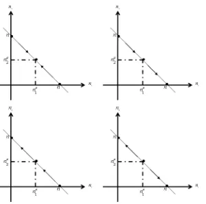
1. The analysis of the stability in the Liapunov sense of the first type of equilibria, give place to the following 4 different cases, see figure (2). Let N′

= (N′ 1, N

′

2) be the distribution after a perturbation in the

equilibrium distribution of the firms:

(i) Consider the case where: (Ne

1, N2e) >> 0 if there exists a

neigh-borhood Vne ⊂ R2 ∩∆_n of (ne₁, ne₂) such that Π_i(y_i∗(n₁, n₂)) <

Πi(y∗(ne1, ne2))i∈ {1,2} ∀(n1, n2)∈ Vne then the dynamical

equi-librium is asymptotically stable, see theorem (1) . (ii) In the others three cases, whereπi(y∗

i(n

′ 1, n

′

2))> πi(y ∗

i(ne1, ne2)) for

at least one i∈ {1,2} the dynamical equilibrium is unstable, see theorem (1) .

6

6 An example 23

Fig. 2: Figure at the top and left, the only case of asymptotically stable equilibrium

2. For the cases on the second type, the dynamical equilibrium is asymp-totically stable if, being

(iii) (Ne

1, N2e) = (1,0) the inequality Π2(yi∗(n

′ 1, n

′

2))<Π1(y∗i(n

′ 1, n

′ 2)) is

verified, or if, (iv) being (Ne

1, N2e) = (0,1) the inequality Π2(yi∗(n

′

1, n′2))>Π1(yi∗(n

′ 1, n′2))

is verified.

Note that for the last case considered in section (4.3) we have that

gj(N) =aj+bj(π∗

j(N)−π

∗

i(N), j 6=i∈ {1,2}and then ifπ

∗

j(N)−π

∗

i(N)>0

it follows thatg(N)Ne_{>0.Then the asymptotical stability of the stationary}

point Ne i =

A B, N

e

j = 1− A

B holds.

6

An example

This example is inspired in ([3]).

Consider a neoclassical private ownership production economy with com-modity space R2 _{havingm consumer divided in two types, m}

1 of type 1 and

m2 of type 2, the setF1 ={1, ...m1}symbolize the consumers of type 1, and

F2 ={(m1+ 1), ..., m}we symbolize the consumers of type 2. Havingnfirms

of two typesn1 of type 1 andn2 of type 2, with the following characteristics:

• Consumers type 1: Initial endowments wi = 1

m1(1,3) and utility

6 An example 24

• Consumers type 2: Initial endowments wi = 1

m2(2,3) and utility

func-tion ui(x, y) = xy2_{, i∈ {(m}

1+ 1), ..., m}.

• Firms type 1: Production set Y1 =

(x, y)∈R2 _{:x <1,and y≤} x x−1 .

• Firms type 2: Production set Y2 ={(x, y)∈R2 :x <1,andy ≤g(x)}

where:

g(x) =







1−ex _{if x≤0}

ln(1−x) if 0< x <1

• Shares: Type 1 consumers have own one third of type 1 firms, and two thirds of type 2, the rest is owned by the consumers of type 2. Within each type, individuals have the same share of firms, i.e:

θi1 = _3m1₁, ∀i∈ F1 and θi2 = _3m2₁, ∀i∈ F2, i= 1, ....m1;

θi1 = _3m2₂, ∀i∈ F1 and θi2 = _3m1₂, ∈ F2, i=m1+ 1, ..., m.

We start considering the supply function of a firms of type 1: The tech-nological set Y1 is strictly convex and the efficiency frontier is

EF F(Y1) =

x, x x−1

, x <1

.

So the profit function of a firm of this type is given by:

π1(x) = p1x+p2

x

x−1. (16) The supply of a firm of type 1, is: x1(p) = 1−

q_p

2

p1. Writing t =

q_p

2

p1 we

obtain that the output input vector is given by

y1(t) =

1−t,1− 1

t

.

Substituting x =y2(t) in (18) we obtain that the profit for a firm of type 1

is: π1(t) =p1(1−t)2.

Remark 1: Note that the rate of profits is given by

Π1(t) =



 

 

π1(t)

−p2(1−1_t) =−1 +

1

t 0< t <1 π1(t)

−p1(1−t) = 1−t 1< t

6 An example 25

For a firm of type 2, we obtain

EF F(Y2) ={(x,1−ex), x≤0} ∪ {(x,ln(1−x), 0< x < 1}.

The profit function is given by:

π2(x) =







p1[x+t2(1−ex)] x≤0

p1[x+t2ln(1−x)] 0< x <1

(18)

since π′′

2(x)<0 in both cases, then the supply of a firm of type 2 is:

y2(t) =







(1−t2_{,2 lnt) if 0< t <1,}

−2 lnt,1−_t12

if t≥1.

Substituting x =y2(t) in (18) we obtain that the profit for a firm of type 2

is:

π2(t) =







p1[(1−t2) + 2t2lnt] if 0< t <1,

p1[−2 lnt+t2−1] if t >1.

Remark 2: Note that the rate of profits of a firm of type 2 is given by:

Π2(t) =







−1+t2

2t2_lnt + 1 if 0< t <1,

−2 lnt+t2₋₁

2 lnt if t >1

(19)

The demand of each consumer of type 1, is given by:

x1(t) =

W1(t)

2p1

1, 1 t2

(20)

and the demand of each consumer of type 2, is given by:

x2(t) =

W2(t)

3p1

1, 2 t2

(21)

Where Wi(t) denotes the income of a consumer of type i at prices p =

p1(1, t2). We shall compute:

6 An example 26

W1(t) =

p1

3m1







(9 +n1+ 2n2)t2−2n1t+ 3 +n1−2n2−4n2lnt if t≥1

(9 +n1−2n2)t2−2n1t+ 4n2t2lnt+ (3 +n1 + 2n2) if 0< t <1

(22)

W2(t) =

p1

3m2







(9 + 2n1+n2)t2−4n1t+ 6 + 2n1−n2−2n2lnt if t≥1

(9 + 2n1−n2)t2−4n1t+ 2n2t2lnt+ 6 + 2n1 +n2 if 0< t <1

(23) Substituting in (20) we obtain the demand for each consumer of type 1:

x1(t) =

                  

(9+n1+2n2)t2−2n1t+3−n1−2n2−4n2lnt,

6m1

(9+n1+2n2)t2−2n1t+3+n1−2n2−4n2lnt

6m1t2

if t≥1,

(9+n1−2n2)t2−2n1t+3+n1+2n2+4n2t2lnt

6m1 ,

(9+n1−2n2)t2−2n1t+3+n1+2n2+4n2t2lnt

6m1t2

if 0< t <1.

(24) and substituting in (21) we obtain the demand for each consumer of type 2:

x2(t) =

              

(9+2n1+n2)t2−4n1t+6+2n1−n2−2n2lnt

9m2 ,2

(9+2n1+n2)t2−4n1t+6+2n1−n2−2n2lnt

9m2t2

if t≥1

(9+2n1−n2)t2−4n1t+2n2t2lnt+6+2n1+n2

9m2 ,2

(9+2n1−n2)t2−4n1t+2n2t2lnt+6+2n1+n2

9m2t2

if 0< t <1

(25) The aggregate excess demand function will be:

6 An example 27

ζ1(t) = ₁₈1







(45 + 7n1+ 8n2)t2+ 4n1t−33−11n1−8n2 −20n2lnt if t≥1

(45 + 7n1+ 10n2)t2+ 4n1t−54 + 16n2t2lnt if 0< t <1

ζ2(t) =−₁₈1_t2







(45 + 7n1+ 8n2)t2+ 4n1t−33−11n1−8n2+ 20n2lnt if t≥1

(45 + 7n1+ 10n2)t2+ 4n1t−54 + 16n2t2lnt if 0< t <1

The equilibrium prices are the solution of the equation ζ(t) = 0. To find the solutions of this equation we consider the following functions:

f : (0,∞)→R and g : (0,1)→R

defined by:

f(t) = (45 + 7n1+ 8n2)t2+ 4n1t−33−11n1−8n2−20n2lnt, (a)

g(t) = (45 + 7n1+ 10n2)t2+ 4n1t−54 + 16n2t2lnt. (b)

(26) Note that f′

(t) = 2(45 + 7n1 + 8n2)t + 4n1 − n220_t > 0 ∀t ≥ 1 and

n1, n2 ≥ 0 this means that f(t) is strictly increasing in the interval [1,∞).

Since f(1) = 12 it follows thatζ(t)6= 0 for eacht >1, and then there is not an equilibrium with t >1.

On the other hand, since limt→0g(t) < 0, and g(1) > 0, ∀(n1, n2) ∈ ∆

there exists at least one equilibrium such that t∗

<1.

Note that Π1(¯t) = Π2(¯t) if and only if ¯t =≈ 0.516691803. This means

that a Walrasian equilibrium is a dynamical equilibrium if and only ifqp∗2

p∗

1 =

t∗ _{= ¯t ≈≈ 0.516691803. This equilibrium corresponds (approximatelly) for}

instance to an economy with n2

1 = 1 and ne2 = 40.

6.1

The dynamics

6 An example 28

given by the following dynamical system: ˙

N1 =φ(π1(y1∗(N1))−π2(y2∗(N1)))N1

˙

N2 =−N˙1

N(t0)∈∆0.

(27)

Hereafter, to avoid confusions we uset to symbolize time, and p=qp1

p2.

So the dynamics along an equilibrium path is given by the ˙

N1 =N1φ(Π1((N))−Π2((N)), 0< t <1

in our case ˙

N1 =N1φ

−2 + 1−p

2_(N 1)

2p2_(N

1) lnp(N1)

+ 1

p(N1)

Note that this equation is decreasing in the interval (0,1) andφ(¯t)≈φ(0.516691803) = 0.

So, if for a distributionN of the firms over the available technologies the inequality t(N)< 0.516691803 then Π1(N1)−Π2(N) > 0 and the quantity

of firms of type 1 increase and then this difference decrease. Contrarily, if

t(N)>0.516691803 then Π1(N1)−P i2(N)<0 and the quantity of firms of

type 2 increase and then this difference increase.

6.2

The transition path

Let us now characterize the trajectory of the economy of our example along a Walrasian equilibrium trajectory.

Consider a regular economy such that in timet =t0

n(t0) =n0 = (n10, n20)

i.e, En10,n20. It is possible to choose a neighborhood and a correspondence

p∗

: ∆∪Un0 →2

R2 +,

such that p∗

(n1,n2) = Eqn1.

Letp∗

(n0) = (p∗1(n10), p∗2(n20))∈p∗(n10, n20) such thatp0 =

q_p∗

1(n10)

p∗

2(n10) <

6 An example 29

From the correspondencep∗

choose a continuous selectionp∗

,such that

p∗

(n0) = p∗(n10, n20).

There exists a neighborhood Vn0) ⊂ ∆∩Un0 such that for all for all

(n1, n2)∈Vn0, p

∗

(n1) verify thatp(n1) =

q_p∗

1(n1)

p∗

2(n1) <0.516691803.

From the implicit function theorem p:Vn0 →Up0 is a smooth function

verifying

dp∗

dn1

(n10) = p

′

n1(n10) =

−3p0+ 4−16p0lnp0

−4n1(p0)3+ 108p−2016(n−n10)

.

The economy En1(t0),n2(t0) evolves along the transition path to an

sta-tionary state, (ne

1, ne2)∈ De being

lim

(n1,n2)→(ne

1,ne2)

p∗

(n1, n2) = p∗(ne1, ne2)≈0.516691803.

Along this transition path a economyEn1 the share of economies of type

1 increases and the economies of type 2, decreases in equal proportion.

An economy En1 is singular if and only if for some p0,

−4n1(p0)3+ 108p−02+ 16(n−n10) = 0.

Given that the initial economy is regular, then all economy in the neigh-borhood Vn0 is regular.

Analogously, it follows that, if the equilibrium for the initial economy, verify that 0.516691803 < p0 <1 then we will observe a contrary evolution,

i.e, the share of firms of type 1 decreases, and increases the share of firms of type 2.

Note that, a Walrasian equilibrium price p∗

(n1, n2) will be, at the same

time, an stationary equilibrium if and only if, there exists a distribution

n = (n1, n2) for which the equalities

π1(p∗(n1, n2)) = π2(p∗(n1, n2)) and ζ(p∗(n1, n2)) = 0

7 Conclusions 30

7

Conclusions

In this paper, we have shown that a dynamical process based on imitation leads to the economy over a trajectory of Walrasian equilibria. Since the equilibrium prices and the corresponding profits depend on the distribution of the firms over the set of available technologies, the hypothesis of rationality implies that each manager (with identical interest than the owner), try to anticipate the behavior of their competitors. This occurs because the future profits will depend on the joint choice of the managers on the set of available technologies.

One of the main questions, that we attempt to answer in this paper, is how or based in what arguments, managers, looking for more profitable investments, decide to maintain or change the actual technology under which their firms are producing. We considered that, under incomplete information, managers follow an imitation process.

As this process imitative process continues, the economy changes, more specifically, the set of Walrasian equilibria changes. The economy evolves along a transition path, which reflects the evolution of the distribution of the firms over the set of available technologies. In this process, the wealth of consumers changes, because their shares on firms change, and thereby the excess demand functions change. Consequently, the economy changes. So, the set of Walrasian equilibria depends on the distribution of the firms, and so, this distribution determines the characteristics of the economies, i.e, if they are regular or singular. The changes in the economy along the transition path, will no longer be continuous in a neighborhood of a singular price. It is for these reasons, that we consider singular economies as the thresholds of economic crises. Only singular economies have associate singular equilibria. Big changes can be expected when the distribution of the firms determines that the economy is in a neighborhood of a singular economy. Therefore, the possibility that an economic crisis happens is a structural phenomenon, that lies at the basis of the model itself, particularly in the assumed rationality of the agents.

References

7 Conclusions 31

Game and Science” (in Honour of Maurcio Peixoto and David Rand) Series: Springer-Veralg. Vol. 2 ch 4. pp. 55-7.

[2] Acemoglu, D. and M.K. Jensen (2013) “Aggregate comparative statics,”

Games and Economic Behavior, 81, 27-49.

[3] Aliprantis C.D., D.J. Brown and O. Burkinshaw (1990) Existence and Optimaility of Competitive Equilibria. Springer Verlag.

[4] Ania, A.B. (2008) “Evolutionary stability and Nash equilibrium in fi-nite populations, with an application to price competition,” Journal of Economic Behavior & Organization, 65, 472-488.

[5] Apesteguia, J., S. Huck, J. Oechssler and S. Weidenholzer (2010) “Imi-tation and the evolution of Walrasian behavior: theoretically fragile but behaviorally robust,” Journal of Economic Theory 145, 1603-1617.

[6] Balasko, Y. (2009) “The Equilibrium Manifold Postmodern Develop-ments in the Theory of General Economic Equilibrium.” The MIT Press.

[7] Ben-Shoham, A., R. Serrano and O. Volij (2004) “The Evolution of Exchange,” Journal of Economic Theory, 114, 310-328.

[8] Bergin, J. and D. Bernhardt (2009) “Cooperation through imitation,”

Games and Economic Behavior, 67-2, 376-388.

[9] Duersch, P., J. Oechssler and B.C. Shipper (2012) “Unbeatable imita-tion,” Games and Economic Behavior, 76, 88-96.

[10] Harrington Jr., J.E. and M.-H. Chang (2005) “Co-evolution of firms and consumers and the implications for market dominance,” Journal of Economic Dynamics & Control, 29, 245-276.

[11] Hirsch, M., S. Smale and R. Devaney (2003) “Differential Equations, Dynamical Systems, and an Introduction to Chaos.” Academic Press (2003).

7 Conclusions 32

[13] Huang, W. (2011) “Price-taking behavior versus continuous dynamic optimizing,” Journal of Economic Behavior & Organization, 78, 37-50.

[14] Kandori, M., Serrano and O. Volij (2004) “Decentralized Trade, Random Utility and the Evolution of Social Welfare,” Working Paper, Depart-ment of Economics, University of Tokyo.

[15] Mas-Colell, A. (1989) “The Theory of General Equilibrium: A Differen-tiable Approach.” Cambridge University Press.

[16] Perla, J. and C. Tonetti (2014) “Equilibrium Imitation and Growth,”

Journal of Political Economy, 122-1, xx-xx.

[17] Schenk-Hopp´e, K.R. (2000) “The evolutuion of Walrasian behavior in oligopolies,” Journal of Mathematical Economics, 33, 35-55.

[18] Schlag, K. (1998) “Why Imitate, and If So, How? A Boundedly Rational Approach to Multi-Armed Bandits,” Journal of Economic Theory, 78, 130-56.

[19] Vega-Redondo, F. (1997) “The Evolution of Walrasian Behavior,”

Econometrica, 65-2, 375-84.