Novel 3D compression methods for geometry, connectivity and texture

Novel 3D compression methods for geometry, connectivity

and texture

SIDDEQ, Mohammed M and RODRIGUES, Marcos

<http://orcid.org/0000-0002-6083-1303>

Available from Sheffield Hallam University Research Archive (SHURA) at:

http://shura.shu.ac.uk/12099/

This document is the author deposited version. You are advised to consult the

publisher's version if you wish to cite from it.

Published version

SIDDEQ, Mohammed M and RODRIGUES, Marcos (2016). Novel 3D compression

methods for geometry, connectivity and texture. 3D Research, 7 (13).

Copyright and re-use policy

See http://shura.shu.ac.uk/information.html

Sheffield Hallam University Research Archive

1

Novel 3D Compression Methods for Geometry, Connectivity and Texture

M. M. Siddeq and M. A. Rodrigues

GMPR-Geometric Modelling and Pattern Recognition Research Group, Sheffield Hallam University, Sheffield, UK

mamadmmx76@yahoo.com, M.Rodrigues@shu.ac.uk

Abstract

A large number of applications in medical visualization, games, engineering design, entertainment, heritage, e-commerce and so on require the transmission of 3D models over the Internet or over local networks. 3D data compression is an important requirement for fast data storage, access and transmission within bandwidth limitations. The Wavefront OBJ (object) file format is commonly used to share models due to its clear simple design. Normally each OBJ file contains a large amount of data (e.g. vertices and triangulated faces, normals, texture coordinates and other parameters) describing the mesh surface. In this paper we introduce a new method to compress geometry, connectivity and texture coordinates by a novel Geometry Minimization Algorithm (GM-Algorithm) in connection with arithmetic coding. First, each vertex (x, y, z) coordinates are encoded to a single value by the GM-Algorithm. Second, triangle faces are encoded by computing the differences between two adjacent vertex locations, which are compressed by arithmetic coding together with texture coordinates. We demonstrate the method on large data sets achieving compression ratios between 87%—99% without reduction in the number of reconstructed vertices and triangle faces. The decompression step is based on a Parallel Fast Matching Search Algorithm (Parallel-FMS) to recover the structure of the 3D mesh. A comparative analysis of compression ratios is provided with a number of commonly used 3D file formats such as VRML, OpenCTM and STL highlighting the performance and effectiveness of the proposed method.

1.

Introduction

Algorithms for 3D data compression and reconstruction are enabling technologies where cheap storage and data transmission over the network are required. Examples of applications can be found in security, engineering, CAD/CAM collaborative design, medical visualisation, entertainment, e-commerce and geographical information systems among others [1]. Concerning geometry and connectivity compression, Rodrigues and Robinson[2] used PDE-Partial Differential Equations to lossycompression and reconstruction of mesh surfaces with no loss of accuracy in the context of 3D face recognition. They proposed that surface patches can be compressed as a 2D image together with 3D calibration parameters, transmitted over a network and remotely reconstructed (geometry, connectivity and texture map) at the receiving end with the equivalent resolution as the original data. Extending that research, Siddeq and Rodrigues [3]proposeda 2D image compression method based on DWT and DCT which has been demonstrated in the context of structured light 3D reconstruction.The method produces anested series of high-frequency matrices which are coded by a Minimize-Matrix-Size Algorithm (MMS).At decompression stage, a Limited-Sequential Search Algorithm (LSS) is used torecover the original 2D image which is then used for 3D reconstruction of the original mesh. The advantagesofthe method arethe recovery of high resolution imageswith compression ratios up to 98%. Although superior to the PDE compression for the same application, the method proved very complex resulting in execution time of the order of minutes for a high resolution image.

2

1.1. Compression for Fast Rendering

In this section we discuss representations of triangle meshes that are used for transmission to graphics hardware. 3D-hardware support is primarily based on the rendering of triangles, specified by its three vertices, where each vertex contains three coordinates, possibly the surface normal, material attributes and/or texture coordinates. The coordinates and normals are specified with floating point values, such that a vertex may contain data of up to 36 bytes. Thus the transmission of a vertex is expensive and the simple approach of specifying each triangle by the data of its three vertices is wasteful as for an average triangle mesh each vertex must be transmitted six times [13].

The introduction of triangle strips helped to save unnecessary transmission of vertices. Two successive triangles in a triangle strip are joined at an edge. Therefore, from the second triangle on, two vertices of the previous triangle can be combined with only one new vertex to form the next triangle. As with each triangle at least one vertex is transmitted and as an average triangle mesh has twice as many triangles as vertices, the maximal gain is that each vertex has to be transmitted only about twice. Two kinds of triangle strips are commonly used – the sequential and the generalized triangle strips. In generalized triangle strips an additional bit is sent with each vertex to specify to which of the free edges of the previous triangle the new vertex is attached. Sequential strips even drop this bit and impose that the triangles are attached alternating. OpenGL [15] evolved from the commonly used standard for graphics libraries allowing generalized triangle strips in earlier versions, but the current version is restricted to sequential strips.

1.2. Maximum Mesh Compression

The strategy for fast rendering described above can also be used for the compression of triangle mesh connectivity. Instead of retransmitting a vertex, a reference is inserted into a compressed representation. If a vertex from the buffer is referenced its index within the buffer enters the compressed representation. In the triangle strips of Evans et al. [14] each vertex appears about 2.5 times. The vertices can be rearranged into the order they appear the first time and only the indices of 1:5n vertices need to be inserted in the compressed representation. One additional bit per triangle is needed to specify whether the next vertex is used the first time or the index of an already used vertex follows. This sums up to about 1+0.75 (log2 n) bits per triangle. The disadvantage of this approach is that the storage needs to grow with the size of the triangulated mesh. The measurements of Deering in [16]show that the generalized mesh approach theoretically consumes between eight and eleven bits per triangle if an optimal stripper is available.

Taubinet al. [17] propose a very advanced global compression technique for the connectivity of triangle meshes. The method is based on a similar optimization problem as for sequential triangle strips and the authors suggest that it is NP-complete. Their approximation allows compression to only two bits per triangle and there exist triangle meshes which consume only one bit per triangle. The decompression splits into several processing steps over the complete mesh, which makes the approach unsuitable to speed up hardware driven rendering.

Our compression technique introduces a new idea for geometry compression by geometry minimization algorithm and the triangle faces (connectivity) encoded by computing the differences between two adjacent vertices and then encodingeach group of connectivity by arithmetic coding. This approach compares favourably with a number of3D data file formats techniques focusing on compression ratio as it is demonstrated in the experimental section of this paper. This paper is organized as follows. Section 2 introduces the Geometry Minimization algorithm (GM-algorithm) applied to vertices. Section 3 describes the texture compression by using soft-quantization with arithmetic coding, also in this section the connectivity (triangle faces) are compressed by computing the differences between two adjacent faces. Section 4 describes the Parallel Fast Matching Search Algorithm (Parallel-FMS) used to reconstruct the vertex data. Section 5 describes experimental results for 3D data compressionand the results are compared with other 3D file formats. Finally, Section 6 provides a summary and a conclusion.

2.

Vertex Compression

3

𝑉)*+= 𝑟𝑜𝑢𝑛𝑑 𝑉)*+ . 𝑆 (1)

By above Eq.(1) yielding a newset of quantized vertices𝑉)*+ = [ 𝑋, 𝑌, 𝑍] where each vertex size is less than

32-bit (i.e. 32-32-bit minimum size to represent (X, Y, Z) while in previous work each axes need at least 16-bit [5], [13]). Additionally, we reduced the number of bits for each vertex to less than 16-bit by calculating the differences between two adjacent coordinates as follows:

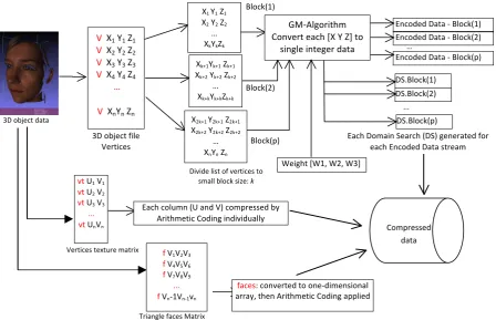
𝐷:= 𝐷:− 𝐷(:=>) (2)

Where i=1, 2, 3... m-1 and m is the size of the list of vertices. The differential process defined in Eq. (2) increases data redundancy and it is applied to each axis independently [3].Thus, these two steps reduce the storage cost of geometry and ensure a sufficient geometric accuracy for most applications.

Fig. 1: The proposed 3D data compression method.

Fig. 1 illustrates the main steps in the proposed method. After the differential process is applied to the vertices, the resulting list is divided into k number of non-overlapping blocks such that each block can be worked independently and in parallel by the GM-Algorithm. This significantly speeds up compression and decompression. The GM-Algorithm is based on defining three weight values (W1, W2 and W3) which are

multiplied by the three vertex coordinates (X, Y, Z) in turn and then summed to a single integer value. Eq (3) defines theEncoded Data by the GM-Algorithm [3] for each triplet of vertex values:

𝐸𝑛𝑐𝑜𝑑𝑒𝑑 𝐷𝑎𝑡𝑎(:)= 𝑊>𝑉) : + 𝑊G𝑉* : + 𝑊H𝑉+ : (3)

Where 𝑉₎, 𝑉_*, 𝑉₊ represent the list of vertices (X,Y,Z) within a block of size k. The weight values (W1, W2 and

W3) are generated by the following algorithm described in pseudo code from the maximum value in the list of

vertices:

𝑀 = max 𝑉), 𝑉*, 𝑉+ +MNO PQ_G,PR,PS % Define M as a function of maximum

𝑊>= 𝑟𝑎𝑛𝑑𝑜𝑚(0,1) % First weight≤1 defined by random between 0 and 1

𝑊G= 𝑊1 + 𝑀 + 𝐹 % F is an integer factor F=1,2,3,…

𝑊H= 𝑀 ∗ 𝑊>+ 𝑀 ∗ 𝑊G ∗ 𝐹

3D object file Vertices

Block(1)

Block(2)

Block(p)

Encoded Data - Block(1) Encoded Data - Block(2)

Encoded Data - Block(p)

DS.Block(1) DS.Block(2) DS.Block(p) … … GM-Algorithm Convert each [X Y Z] to

single integer data

X1 Y1 Z1

X2 Y2 Z2

… XkYkZk

Xk+1Yk+1 Zk+1

Xk+2 Yk+2 Zk+2

… Xk+kYk+kZk+k

X2k+1 Y2k+1 Z2k+1

X2k+2 Y2k+2 Z2k+2

… XnYn Zn 3D object data

V X1 Y1 Z1

V X2 Y2 Z2

V X3 Y3 Z3

V X4 Y4 Z4

…

V XnYn Zn

Divide list of vertices to small block size: k

vt U1 V1

vt U2 V2

vt U3 V3

... vt UnVn

Weight [W1, W2, W3]

Each column (U and V) compressed by Arithmetic Coding individually

Vertices texture matrix _{f V} 1V2V3

f V4V5V6

f V7V8V9

... f Vn-1Vn-1vn

Triangle faces Matrix

faces: converted to one-dimensional array, then Arithmetic Coding applied

Compressed data

4

The following Fig. 2 illustratesthe Algorithm applied to a sample of vertices. After applying the GM-Algorithm, the likelihood for each block of vertices is selected from which a Domain Search (DS) is generated to be used in the decompression stage as illustrated in Fig. 3 with a numerical example.

Fig.2: Sample of vertices compressed by GM-Algorithm

Fig. 3: Domain Search (DS) generatedfrom a block of vertices

3.

Texture Mapping Encoding (UV) and Mesh Connectivity Encoding

In order to allow polygons in a 3D structure to be painted from a 2D image a mapping is required. This map is defined by the normalized horizontal and vertical components (u,v) of an image corresponding to each polygon in 3D. A 3D object in model space [23]and corresponding (u,v) mapping is shown in Fig 4(a). In our proposed compression algorithm, the (u,v) texture coordinates are compressed as lossy data in two steps.First, the (u,v) map is quantized by shifting the floating point to integer, i.e. Eq(1). We adopted a shift value of 1000, meaning that each value (u,v) is in the range {8-bit and 16-bit}. Second, the differences between two adjacent data are computed by Eq(2)applied to each axis independently as shown in Fig. 4(b).Finally, arithmetic coding is applied to each (u,v)independently to produce a stream of bits.

(a) (b)

Vertices: after differential process X Y Z

-4 0 0 -3 0 1 -2 0 1

. . .

-2 0 2

GM-Algorithm With Key2

-4, 0, -3, 1, -2, …, 2 Encoded Data

Generate Domain Search (DS) Sample of vertices (before coding)

-101.284 48.426 45.478 -100.916 48.399 45.468 -100.636 48.414 45.426 -100.396 48.449 45.341 -100.150 48.480 45.215 -99.900 48.510 45.053 -99.6262 48.529 44.863 -99.355 48.548 44.653

Quantized vertices -1013 484 455 -1009 484 455 -1006 484 454 -1004 484 453 -1002 485 452 -999 485 451 -996 485 449 -994 485 447

Differential Eq. applied GM-Algorithm applied

-4 0 0 -0.4

-3 0 1 42.9

-2 0 1 43

-2 -1 1 35.9

-3 0 1 42.9

-3 0 2 86.1

-2 0 2 86.2

-994 485 447 -994 485 447

Subtract each column by Eq(2); then apply the GM-Algorithm, maximum value M=|4|, F=1:- Key1=0.1, Key2=7.1, Key3=43.2

Differential Process Eq(2) applied on each U and V

Each of U and V Shift to integer

U V

Arithmetic Coding

Vertices texture consist of; U and V axes

Vt 0.23 0.23 Vt 0.34 0.45 Vt 0.91 0.47

5

Fig. 4: (a) Texture in UV space related to 3D object, (b) UV texture mapping compression

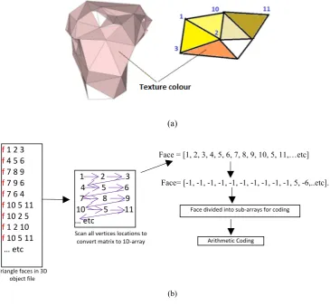
Triangle faces represent geometric connectivity. In a 3D OBJ file, each face contains the vertex indices in the order they appear in the file, normally arranged in ascending order. Triangular faces and vertex indices are illustrated in Fig. 5(a). The advantage of this representation is that each triangle can be compressed in just a few bits. In our proposed method, triangle faces are compressed by applying the differential process defined in Eq. (2). The faces are scanned row-by-row and representedas a one-dimensional array, and the final encoded array is compressed by arithmetic coding. The texture of each triangular face is represented by their (u,v) map which maps a pixel value in the image to a vertex in the 3D structure. Each value in the (u,v) map is normalised and shifted to integer. Texture values are separated from vertex indices (triangle face),they are both compressed in same way as illustrated in Fig. 5(b)

(a)

(b)

Fig. 5(a) 3D mesh represented as vertex indices in a 3D OBJ file; (b) In our method, differential vertex indices are lossless compressed by arithmetic coding.

4.

Decompression Algorithm by Parallel Threads on Blocks of Data

The GM-Algorithm described in Section 2 compresses each vertex data (X, Y, Z) to a single integer value by three different weights (W1, W2, W3). Here we described how to recover the original data.To this purpose we

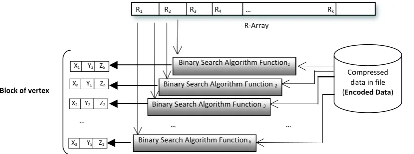
designed a parallel algorithm named Parallel Fast-Matching-Search Algorithm (Parallel-FMS). The header of the compressed file contains information about the compressed data pertaining the weights and DS(the Domain Searchfor each block of vertex as in Fig. 2) followed by streams of compressed encoded data (Encoded Data).

The Parallel-FMS algorithm picks up in turn each k-encoded data to reconstruct k blocks of vertices (X, Y, Z). The Parallel-FMS is based on a binary search algorithm illustrated through the following steps (A) and (B):

Arithmetic Coding

Triangle faces in 3D object file

Scan all vertices locations to convert matrix to 1D-array f 1 2 3

f 4 5 6

f 7 8 9

f 7 9 6

f 7 6 4

f 10 5 11

f 10 2 5

f 1 2 10

f 10 5 11 … etc

Face = [1, 2, 3, 4, 5, 6, 7, 8, 9, 10, 5, 11,…etc]

Face= [-1, -1, -1, -1, -1, -1, -1, -1, -1, -1, 5, -6,..etc].

Face divided into sub-arrays for coding

6

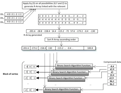
A) Initially, the Domain Sarch (DS)is copied to three separate arrays to estimate X, Y and Z respectively. The searching algorithm computes all possible combinations of X with W1, Y with W2and Z with W3

that yield a result R-Array. As a means of an example consider that DS(1)=[X1 X2 X3] , DS(2)=[Y1 Y2 Y3] and DS(3)=[Z1 Z2 Z3]. Then, according to Eq.(5) these represent VX, VY and VZ respectively. The

equation is executed 27 times to build the R-Array, as described in Fig. 6(a). The match indicates that the unique combination of X, Y and Z represents the orginal vertex block.

B) Abinary search algorithm[22] is used to recover an item in the array. Here we designed a parallel binary search algorithm consisting of k-binary search algorithms working in parallel to reconstruct

kblock of vertices in the list of vertices, as shown in Fig. 6(b). In each step in the k-binary search algorithm compares k-encoded data (i.e. each binary search algorithm takes a single compressed data item) with the middle of the element of the R-Array. If the values match, then a matching element has been found and its R-Array's relevant (X,Y,Z) returned. Otherwise, if the search is less than the middle element of the R-Array, then the algorithms repeats its action on the sub-array to the left of the middle element or, if the value is greater, on the sub-array to the right. All k-binary search algorithms are synchronised such that the correct vertices values are returned. To illustrate our decompression algorithm, the compressed samples in Fig. 2 (by our GM-Algorithm) can be used by our decompression algorithm to reconstruct X, Y and Z values as shown in Fig. 7.

(a) Compute all the probabilities for all possible k-encoded datafor each block of vertices size k

(b) All Binary Search algorithms work in parallel to find a group of decompressed data approximately at same time.

Fig. 6: Parallel-FMS algorithm to reconstruct the reduced array. (a) Compute all the probabilities for all possible

k-Encoded Data (R-Array) by using Weight combinations with DS. (b) All Binary Search Algorithms run in Parallel to recover the decompressed vertices data approximately at same time.

R-Array

Binary Search Algorithm Function 3

Compressed data in file (Encoded Data) Binary Search Algorithm Function 2

Binary Search Algorithm Function1

Binary Search Algorithm Function k

R1 R2 R3 R4 … Rk

X1 Y2 Z5

Xn Y1 Zn

X2 Y2 Z2

X3 Y5 Z1

Each Binary Search find Location of the "R-Array" corresponding to the compressed data, output is relevant [X,Y,Z], which represents a vertex in a block

… _{… …}

Block of vertex

Apply Eq.(3) on all possibilities (X,Y and Z) to generate R-Array linked with the relevant

R-Array

Sort R-Array ascending order X1 X2 X3 X4 X5 X6 … Xk

Y1 Y2 Y3 Y4 Y5 Y6 … Yk

Z1 Z2 Z3 Z4 Z5 Z6 … Zk

DS1

DS2

DS3

R1 R2 R3 R4 … Rk

X1 Y2 Z5

Xn Y1 Zn

X2 Y2 Z2

7

Fig. 7: All Binary Search Algorithm run in Parallel to recover the decompressed vertices data approximately at same time.

Once vertices are recovered, we turn our attention to decoding triangle faces and vertex texture coordinates. The differential process of Eq. (2) is reversed by addition such that the encoded values in each triangle face and texture coordinates return to their original values. This process takes the last value at position m, and adds it to the previous value, and then the total adds to the next previous value and so on. The following equation defines the addition decoder [3].

𝐴(:X>)= 𝐴(:X>)+ 𝐴(:) (4)

where

i= m, (m-1), (m-2), (m-3),…,2.

5.

Experimental Results

The experimental results described here were implemented in MATLAB R2013a and Visual C++ 2008 running on an AMD Quad-Core microprocessor. We describe the results in two parts: first, we apply the compression and decompression algorithms to 3D data object generated by the GMPR 3D surface scanner [2, 18, 19].The principle of operation of GMPR 3D surface scanning is to project patterns of light onto the target surface whose image is recorded by a camera. The shape of the captured pattern is combined with the spatial relationship between the light source and the camera, to determine the 3D position of the surface along the pattern [20] as shown in Fig, 8(a). Second, we apply the method to general 3D object data (i.e. 3D object generated by 3Dmax, CAD/CAM, 3D camera or other devices/software) as shown in Fig. 8(b).

Table 1 show our compression algorithm applied on each 3D object file, and Fig. 9, 10, 11, 12, 13, 14, 15 shows the visual properties of the decompressed 3D object data for 3D images respectively. Additionally, RMSE are used to compare between 3D original object file content (geometric (X, Y, Z) and (u,v) texture coordinates) and the recovered 3D object file content. Root Mean Square Error (RMSE) is used to refer to image quality

-4 0 -3 1 -2 -1 2 -4 0 -3... 2 -4 .... 2 -4 0 -3 1 -2 -1 2

-4 0 -3 1 -2 -1 2 -4 0 -3 1 -2 -1 2 DS1

DS2

DS3

-201.6 -173.2 -158.4 -130 -115.2 ... -0.4 ... 100.8 Apply Eq.(3) on all possibilities (X,Y and Z) to

generate R-Array linked with the relevant

-4 -4 -4 -4 -4 -4 -4 0 0 0... 0 -3... 2 -4 -4 -4 -4 -4 -4 -4 -4 -4 -4...-4 -4 ... 2

-201.6 -28.8 -158.4 14.4 -115.2 -72 57.6 -173.2 -0.4 -130

Sort R-Array ascending order R-Array generated

-0.4 42.9 43 35.9 42.9

86.1 86.2

Binary Search Algorithm Function 3

Binary Search Algorithm Function 2

Binary Search Algorithm Function1

Binary Search Algorithm Function 7

-4 0 0

-3 0 1

-2 0 1

-2 0 2

… _{… …}

Block of vertex

8

mathematically [24, 25]; it can be calculated by computing the differences between the decompressed 3D object and the original 3D object.

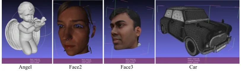
(a) 3D objects created by 3D scanner and 3D software developed by GMPR

Angel Face2 Face3 Car

(b) 3D objects created by other scanning methods and3Dmodel building software Fig. 8: (a) and (b): 3D objects tested by our compression and decompression algorithm

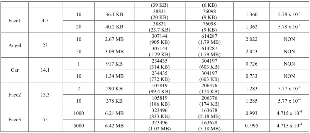
Table 1. Compression and decompression results by the proposed method

3D image

Name Original file size (MB) Shift value Compressed file size

No. of Vertices (Compressed Size)

No. of Triangle faces (Compressed size)

3D RMSE

(X,Y and Z) (Texture UV)2D RMSE

Corner 2.91

1 19.1 KB _{(11 KB)}24168 _{(4 KB)}46878 1.034 _{5.77 x 10}-4

10 32.5 KB _{(24 KB)}24168 _{(4 KB)}46878 1.035 _{5.77 x 10}-4

Metal 5.34 10 36.7 KB

43932 ) KB

(23 (6 KB)86330 1.0618 5.78 x 10-4

50 53.2 KB 43932 86330 1.061 5.78 x 10-4

2D images created by 3D Scanner developed by GMPR

3D scanner based on structured light patterns

3D objects created by 3D surface software created by

GMPR Corner

Metal

9

) KB

(39 (6 KB)

Face1 4.7

10 36.1 KB ₍₂₀ 38831_{KB) (9 KB)}76098 1.360 _{5.78 x 10}-4

20 40.2 KB _(23.7 38831_{KB) (9 KB)}76098 1.362 _{5.78 x 10}-4

Angel 23

10 2.67 MB _{(905 KB)}307144 _{(1.79 MB)}614287 2.022 NON

50 3.09 MB _{(1.29 KB)}307144 _{(1.79 MB)}614287 2.023 NON

Car 14.1 1 917 KB

234435

(314 KB) (603 KB)304197 0.726 NON

10 1.34 MB _{(772 KB)}234435 _{(603 KB)}304197 0.733 NON

Face2 13.3

2 290 KB _{(99.4 KB)}105819 _{(174 KB)}206376 1.283 _{5.77 x 10}-4

10 378 KB _{(186 KB)}105819 _{(174 KB)}206376 1.285 _{5.77 x 10}-4

Face3 55

1000 6.21 MB _{(833 KB)}323496 _{(5.18 MB)}163678 0.993 4.715 x 10-4

5000 6.42 MB _{(1.02 MB)}323496 _{(5.18 MB)}163678 0. 995 4.715 x 10-4

Table 2. Compression and Decompression execution time by the proposed method

3D image Name

Original file

size (MB) Shift value

Estimated Compression Time (sec.)

Estimated Decompression Time (sec.) Vertices

(X, Y, Z)

Triangle faces and texture

Vertices

(X, Y, Z) Triangle faces and texture

Corner 2.91 ₁₀ 1 1.5 _1.9 34.8 _34.4 2.25 _2.35 40.2 _39.1

Metal 5.34 10 2.8 63.5 5.1 70

50 3 64.48 5.4 70

Face1 4.7 10 ₂₀ 2.2 _2.2 54.1 _56.2 4.42 _4.39 65 ₆₆

Angel 23 10 ₅₀ 210.4 _{420.4 355.98} 370.8 _828.89 316.8 400 ₄₀₉

Car 14.1 ₁₀ 1 _180.2 40 176.6 _169.9 71.48 _338.2 210 ₂₀₀

Face2 13.3 ₁₀ 2 25.5 _{10 162.46} 160.4 47.89 _18.5 200 ₂₀₀

10

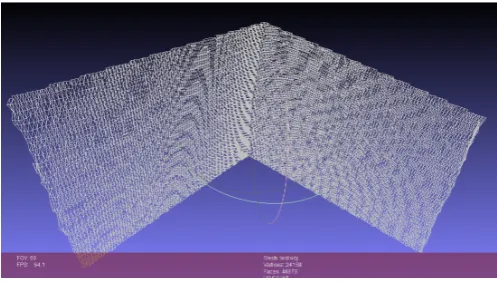
(a) (left) 3D Corner object with texture, (right) 3D mesh Corner shows the details of the object, at compresses size : 32.5 KB

(b) (left) 3D Corner’s vertices organized as structure lines at compression size: 32.5 KB, (right) shows vertices for 3D corner at compression size:19.1 KB, the verticesmoved slightly from their original position.

(c) 3D mesh corner shows the details of the object, at compresses size: 19.1 KB, the image shows the trianglesslightly more degraded than in previous result.

Fig. 9, (a), (b) and (c) shows the decompressed 3D Corner image at compression size: 32.5 KBand 19.1 KB

11

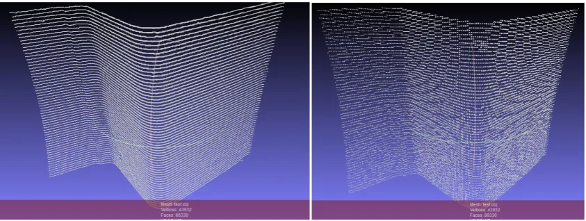
(b) (left) 3D Metal’s vertices organized as structure lines at compression size: 53.2 KB, (right) shows vertices for 3D corner at compression size:36.7 KB, some vertices moved to up and down from their original position.

(c) 3D mesh details of the object, at compresses size: 36.7 KB, the image shows similar high quality 3D mesh surface as in previous result.

Fig. 10: (a), (b) and (c) shows the decompressed 3D Metal image at compression size: 53.2 KBand 36.7 KB

12

(d) (left) 3D Face1 vertices organized as structure lines at compression size: 40.2 KB, (middle) shows vertices for 3D Face1 at compression size: 36.1 KB, the vertices in both 3D images approximately at same original positions. (right) 3D mesh Face1 shows the details of the object, at compresses size: 36.1 KB, the image shows same high

quality as 3D mesh in previous result.

Fig. 11: (a) and (b) shows the decompressed 3D Face1 image at compression size: 40.2 KBand 36.1 KB

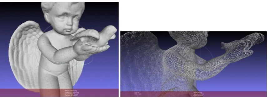
(a) (left) 3D Angel object, (right) 3D mesh Angel shows the details of the object, at compresses size: 3.09 MB

(b) (left) 3D Angel object, (right) 3D mesh Angel shows the details of the object, at compresses size: 2.67 MB, similar from the 3D mesh in previous result

13

(a) (left) 3D mesh Car object, (right) 3D mesh Inside the Car, shows the details of the object, at compresses size: 1.34 MB

(b) 3D mesh Car shows the details of the object, at compresses size: 917 KB, the image shows the vertices for some objects move slightly away from their original positions.

Fig. 13: (a) and (b) shows the decompressed 3D Car image at compression size: 1.34 MB and 917 KB

14

(b)

Fig. 14: (a) and (b) shows the decompressed 3D Face2 image at compression size: 378 KBand 290 KB

(a) Full 3D texture Face3 object, shows the details of the object, at compresses size: 6.42 MB

(b) (left) 3D mesh shows the details of the 3D Face3, at compresses size: 6.42 MB, (right) 3D mesh at compressed size 6.21 MB, the vertices slightly move away from their original positions.

Fig. 15: (a) and (b) shows the decompressed 3D Face3 image at compression size: 6.42 MB and 6.21 MB

15

Table 3. Our approach compared with other encoding 3D data format

Method

3D Object file

Corner (Original file size 2.91 MB) Metal (Original file size 5.34 MB) Face1 (Original file size 4.7 MB)

Angel (Original file size 23.5 MB) Car (Original file size 14.1 MB)

Face2 (Original file size 13.3 MB)

Face3 (Original file

size 55 MB)

Proposed Method

Compressed

file size 32.5 KB 53.2 KB 40.2 KB 2.02 MB 1.34 MB 378 KB 6.42 MB Compression

ratio 98.9% 99% 99.1% 91% 90.4% 97.2% 88.3%

MATALB Format

Compressed

file size 850 KB 1.53 MB 1.32 MB 5.31 MB 4.4 MB 4.04 MB 11.9 MB Compression

ratio 71.4 % 71.3% 71.9% 77.4% 68.7% 69.6% 78.3%

VRML Format

Compressed

file size 2.39 MB 4.43 MB 3.9 MB 23.2 MB 13.7 MB 9.19 MB 17.5 MB

Compression

ratio 17.8% 17% 17% 1.27% 2.9% 30.9% 68%

STL Format

Compressed

file size 2.23 MB 4.11 MB 3.62 MB 29.2 MB 14.5 MB 9.84 MB 15.4 MB Compression

ratio 6.69% 23% 22.9% NON NON 26% 72%

OpenCTM Format

Compressed

file size 145 KB 220 KB 176 KB 1.92 MB 1.36 MB 808 KB 789 KB

Compression

ratio 95% 95.9% 96.3% 91.6% 90.3% 94% 98.5%

6.

Conclusion

This research has presented and demonstrated a new method for 3D data compression/reconstruction and compared the quality of compression through 3D reconstruction, 3D RMSE and the perceived quality of the 3D visualisation. The method is based on converting geometric values to a stream of encoded integer data by the GM-algorithm. Connectivity data are partitioned into groups where each group is addressed by arithmetic coding for lossless compression. The results demonstrate that our approach yields high quality 3D compression at higher compression ratios compared with other 3D data formats. Although the lossy compression controlled by the shift parameter introduces small reconstruction errors as observed by RMSE and detailed visualization,the methods provide high compression ratios with high quality data and it is appropriate for most applications, including demanding applications such as 3D face recognition. A disadvantage of the method is the large number of steps for compression and decompression. The main bottleneck is related to theParallel-FMS algorithm leading to increased execution time through a binary search method. Methods to speed up execution are being investigated and will be reported in the near future.

References

[1] M. Rodrigues, A. Osman and A. Robinson(2011). Efficient 3D data compression through parameterization of free-form surface patches. In: Signal Process and Multimedia Applications

(SIGMAP), Proceedings of the (2010) International Conference on. IEEE, 130-135.

[2] M. Rodrigues, A. Osman and A. Robinson, (2013a) Partial differential equations for 3D data compression and reconstruction, Journal Advances in Dynamical Systems and Applications, Vol. 8 No. 2, 303-315.

[3] M. M. Siddeq, M. A. Rodrigues(2014) A Novel Image Compression Algorithm for high resolution 3D Reconstruction, 3D Research. Springer Vol. 5 No.2.DOI 10.1007/s13319-014-0007-6

[4] Peng, J., C. S. Kim, C., C. Kuo (2005). Technologies for 3D mesh compression: A survey. Journal of

Visual Communication and Image Representation16(6) (2005) 688–733.

[5] Jarek Rossignac (2003) 3D mesh compression. College of Computing and GVU Center Georgia institute of Technology Report, june 2003 Chapter Five- Visualization HandBook.

16

[7] Deering, M. (1995). Geometry Compression, SIGGRAPH 95 Proceedings of the 22nd Annual

Conference on Computer Graphics and Interactive Techniques.

[8] Taubin, G., Horn, W., Lazarus, F., Rossignac, J. (1998), Geometry coding and VRML, Proceedings of The IEEE, 86(6).

[9] Hollinger, S.Q., A.B. Williams, and D. Manak (1998). 3D data compression of hyper spectral imagery using vector quantization with NDVI-based multiple codebooks, IEEE International Geosciences and

Remote Sensing Symposium IGARSS’98, volume 5, 2680–2684.

[10] Shikhare, D., S.V. Babji, and S.P. Mudur (2002). Compression techniques for distributed use of 3D data: an emerging media type on the internet, 15th International Conference on Computer

Communication, India, pp 676–696.

[11] Taubin, G. and J. Rossignac(1998), Geometric compression through topological surgery, ACM Trans. Graph. 17 (2), pp. 84-115.

[12] Szymczak, A., D. King and J. Rossignac (2000). An Edgebreaker-Based Efficient Compression Scheme for Regular Meshes, 12th Canadian Conference on Computational Geometry, pp 257–265.

[13] Topraj Gurung, Mark Luffel, Peter Lindstrom, Jarek Rossignac (2013), Zipper: A compact connectivity data structure for triangle meshes. Journal of Computer –Aided Design Vol 45. No.2, pp. 262-269

[14] 3DCT (2012). 3D Compression Technologies (3DCT), www.3dcompress.com/web/default.asp, accessed Oct 2012.

[15] Francine Evans, Steven S. Skiena, and Amitabh Varshney (1996). Optimizing triangle strips for fast

rendering. In IEEE Visualization. IEEE, October 1996. ISBN 0-89791-864-9.

[16] Jackie Neider, Tom Davis, and Mason Woo (1997). OpenGL Programming Guide —The Official

Guide to Learning OpenGL, Version 1.1. Addison-Wesley, Reading, MA, USA.

[17] M. Deering (1995). Geometry compression. In Computer Graphics (SIGGRAPH ’95 Proceedings), pp. 13–20.

[18] Gabriel Taubin and JarekRossignac (1996). Geometric compression through topological surgery. Technical report, Yorktown Heights, NY 10598, January 1996. IBM Research Report RC 20340.

[19] M. Rodrigues, M. Kormann, C. Schuhler and P. Tomek (2013b) Robot trajectory planning using OLP and structured light 3D machine vision. Lecture notes in Computer Science Part II. LCNS Springer, Heidelberg, Vol. 8034, pp 244-253.

[20] M. Rodrigues, M. Kormann, C. Schuhler and P. Tomek (2013c). Structured light techniques for 3D surface reconstruction in robotic tasks

.

Recognition Systems CORES 2013, Springer, pp. 805-814.

[21] M. Rodrigues, M. Kormann, C. Schuhler and P. Tomek (2013d). An intelligent real time 3D vision

system for robotic welding tasks. In: Mechatronics and its applications. IEEE Xplore, pp. 1-6.

[22] Knuth, Donald (1997). Sorting and Searching: Section 6.2.1: Searching an Ordered Table, The Art of Computer Programming 3 (3rd Ed.), Addison-Wesley. pp. 409–426. ISBN 0-201-89685-0

[23] Murdock, K.L. (2008). 3DS Max 2008 Bible. 1st ed. Indianapolis, Indiana: Wiley Publishing, Inc. ISBN 9780470417584

.

[24] I.E. G.Richardson(2002) VideoCodecDesign, JohnWiley&Sons.

[25] K.Sayood, (2000) Introduction to Data Compression, 2nd _{edition, Academic Press, Morgan Kaufman}