JIT Based cost analysis for dynamic program transformations

JIT-Based cost analysis for dynamic program

transformations

MORTON, John Magnus, MAIER, Patrick

<http://orcid.org/0000-0002-7051-8169> and TRINDER, Phil

Available from Sheffield Hallam University Research Archive (SHURA) at:

http://shura.shu.ac.uk/18622/

This document is the author deposited version. You are advised to consult the

publisher's version if you wish to cite from it.

Published version

MORTON, John Magnus, MAIER, Patrick and TRINDER, Phil (2016). JIT-Based cost

analysis for dynamic program transformations. Electronic Notes in Theoretical

Computer Science, 330, 5-25.

Copyright and re-use policy

See

http://shura.shu.ac.uk/information.html

Sheffield Hallam University Research Archive

JIT-Based Cost Analysis for Dynamic Program

Transformations

John Magnus Morton

Patrick Maier

Phil Trinder

School of Computing Science Univeristy of Glasgow

UK

Abstract

Tracing JIT compilation generates units of compilation that are easy to analyse and are known to execute frequently. The AJITPar project investigates whether the information in JIT traces can be used to dynam-ically transform programs for a specific parallel architecture. Hence a lightweight cost model is required for JIT traces.

This paper presents the design and implementation of a system for extracting JIT trace information from the Pycket JIT compiler. We define three increasingly parametric cost models for Pycket traces. We determine the best weights for the cost model parameters using linear regression. We evaluate the effectiveness of the cost models for predicting the relative costs of transformed programs.

Keywords: Cost Model, JIT Compiler, Program Transformation, Skeleton, Parallelism

1

Introduction

The general purpose hardware landscape is dominated by parallel architectures — multicores, manycores, clusters, etc. Writing performant parallel code is non-trivial for a fixed architecture, yet it is much harder if the target architecture is not known in advance, or if the code is meant to be portable across a range of architectures. Exist-ing approaches to address this problem ofperformance portability, e.g. OpenCL [21], offer device abstraction yet retain a rather low-level programming model typically intended for a specific problem domain, e.g. for numerical data-parallel problems.

There is less language support for multiple architectures in other domains. For example symbolic computations, like combinatorial searches or computational al-gebra, often exhibit large degrees of parallelism but the parallelism is irregular:

1

Email:[email protected]

2

Email:[email protected]

3

Email:[email protected]

4

This work is funded by UK EPSRC grant AJITPar (EP/L000687/1).

Electronic Notes in Theoretical Computer Science 330 (2016) 5–25

1571-0661/© 2016 Published by Elsevier B.V.

www.elsevier.com/locate/entcs

http://dx.doi.org/10.1016/j.entcs.2016.12.012

the number and size of parallel tasks is unpredictable, and parallel tasks are often created dynamically and at high rates [28].

TheAdaptive Just-in-Time Parallelism(AJITPar) project [2] investigates a novel approach to deliverportable parallel performance for programs with irregular paral-lelism across a range of architectures by combining declarative task paralparal-lelism with dynamic scheduling and dynamic program transformation. Specifically, AJITPar proposes to adapt task granularity to suit the architecture by transforming tasks at runtime, thus varying the amount of parallelism depending on the architecture. To facilitate dynamic transformations, AJITPar will leverage the dynamic features of the Racket language and its recent trace-based JIT compiler, Pycket [13,10].

Dynamic task scheduling and task transformation both benefit from predicted task runtimes. This paper investigates how to construct lightweight cost models for JIT traces. A JIT trace is simply a linear path through the program control flow graph that the compiler has identified as being executed often. We hypothesize that even very simple cost models can yield sufficiently accurate predictions as traces have very restricted control flow, and we only require to compare the relative costs of pre- and post-transformed expressions.

The main contributions in this paper are as follows. We have designed and imple-mented a system for extracting JIT trace information from the Pycket JIT compiler (Section3). We have defined 3 cost models for JIT traces, ranging from very simple to parametric, and we have used an regression analysis over the Pycket benchmark suite to automatically tune the architecture-specific cost model parameters (Sec-tion4). We have shown that the tuned cost model can be used to accurately predict the relative execution times of transformed programs (Section5).

2

Related Work

2.1 AJITPar

and trace-based JIT compilers build intermediate data structure (traces) that may be costed.

The work described in this paper aims to identify a system for calculating relative costs of traces, which will be used to determine the scheduling of parallel tasks based on their relative costs, and the selection of appropriate transformations to optimise for the parallel work available in the task.

2.2 Tracing JIT

Interpreter-based language implementations, where a program is executed upon a virtual machine rather than on a real processor are often used for a variety of reasons - including ease of use, dynamic behaviour and program portability, but are often known for their poor performance compared to statically compiled languages such as C or FORTRAN.

JIT compilation is a technology that allows interpreted languages to significantly increase their performance, by dynamically compiling well-used parts of the pro-gram to machine code. This enables interpreters or virtual machine languages to approach performance levels reached by statically compiled programs without sac-rificing portability. Dynamic compilation also allows optimisations to be performed which might not be available statically.

JIT compilation does not compile the entire program as it is executed, rather it compiles small parts of the program which are executed frequently (these parts are described as hot). The most common compilation units are functions (or methods) and traces [8]. A trace consists of a linear sequence of instructions which make up a single iteration of the body of loop. A complete trace contains no control-flow except at the points where execution could leave the trace; these points are known asguards. The main benefit of traces compared to functions as a unit of compilation is that it can form the entire body of a loop spanning multiple functions, rather than just the body of a single function.

2.3 RPython Tool-chain

The specific JIT technology we use is part of the RPython tool-chain. PyPy [32] is an alternative implementation of the Python programming language [33], notable for having Python as its implementation language. PyPy is implemented using a subset of the Python language known as RPython and the tool-chain is intended to be used as a general compiler tool-chain. Smalltalk [12] and Ruby [39] are examples of languages implemented on the RPython tool-chain. PyPy has a trace-base JIT, and the RPython tool-chain allows for the JIT to be easily added to a new interpreter implementation

AST.

JITs built with RPython are notable in that they aremeta-tracing [11]. Rather than trace an application level loop, the JIT traces the actual interpreter loop itself. The interpreter will annotate instructions where an application loop begins and ends in order for appropriate optimisations to be carried out. The purpose of this is so that compiler writers do not need to write a new JIT for every new language that targets RPython/PyPy, they just provide annotations.

2.4 Cost Analysis

Resource analysis is important in resource-limited systems like most embedded sys-tems, in hard real-time systems where timing guarantees are required, and for direct-ing program refactordirect-ing or transformation. Here we seek a static resource analysis to inform dynamic program transformations. Recently there has been significant progress in both the theory and practice of resource analysis. Some of this progess is reported in the FOPARA workshops [19] and the TACLe EU COST action [38].

Analysis techniques exist for a range of program resources, for example execution time [41,1,34], space usage [36,26], or energy [22]. The resource of interest here is predicted execution time. For many applications, e.g. embedded and real-time software systems, the most important performance metric is worst case execution time. Various tools [41,20,1] have been built to statically estimate or measure this; an example is aiT [20] which uses a combination of control flow analysis and lower level tools, such as cache and pipelining analysis. Cache and pipelining analysis attempts to predict the caching and processor pipelining behaviour of a program and is performed in aiT using abstract interpretation. Here however we predict expected, rather than worst case execution time. Moreover we do not need precise absolute costs: approximate relative costs should suffice to allow the transformation engine to select between alternative rewrites.

A range of analysis techniques are used to estimate the resources used by pro-grams. High level cost analysis can be performed on the syntactic structure of the source code of a program, e.g. using a mathematical function of C syntactic constructs to estimate execution time [15]. Low-level representations of code and bytecode can be used as source for static resource analysis [3,4,26,7,6]. For example the COSTA tool [4] for Java which allows the analysis of various resources using parameterized cost models, and the CHAMELEON tool [7] which builds on this approach and uses it to adapt programs.

There are many other approaches in cost analysis including amortized resource analysis [23,6], incremental resource analysis [5], and attempting to enforce resource guarantees usingproof-carrying code [6,9] (the MOBIUS project is a prime example). Control flow is a key element of many resource analyses [41,20]. However, as JIT traces do not contain any control flow, these types of analysis are redundant and a far simpler approach will suffice. This is fortunate as the static analysis must run fast as part of the warm-up phase of the execution of the JIT compiled program.

2.5 Code Transformation

Program transformations are central to optimising compilers. GHC, for instance, aggressively optimises Haskell code by equational rewriting [24,25]. Transformations can also be used for optimising for parallel performance. Algorithmic skeletons [17] – high level parallel abstractions or design patterns – can be tuned by code trans-formations to best exploit the structure of input data or to optimise for a particular hardware architecture. Examples of this include the PMLS compiler [35], which tunes parallel ML code by transforming skeletons based on offline profiling data, and the Paraphrase Project’s refactorings [16] and their PARTE tool for refactoring parallel Erlang programs [14]. PMLS is an automatically parallelising compiler for Standard ML which turns nested sequential higher-order-function calls into parallel skeleton calls and performs code transformation based on runtime behaviour of sub-parts of the program; unlike AJITPar, these transformations are entirely offline and no attempt is made to solve the problem of performance portability. PARTE uses refactoring to allow the introduction of parallel skeletons and the transformation of existing parallel skeletons; these refactorings are applied entirely ahead-of-time and at the instruction of the user, while the transformations are driven by offline profiling.

3

Language Infrastructure

3.1 Pycket Trace Structure

A JIT trace consists of a series of instructions recorded by the interpreter, and a trace becomeshot if the number of jumps back to the start of the trace (or loop) is higher than a given threshold, indicating that the trace may be executed frequently and is worth compiling.

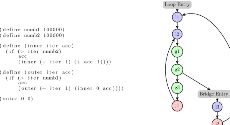
Other important concepts in Pycket traces includeguards: assertions which cause execution to leave the trace when they fail; bridges: that are traces starting at a guard that fails often enough; and trace graphs: representing sets of traces. The nodes of a trace graph are entry points (of loops or bridges), labels, guards, and jump instructions. The edges of a trace graph are directed and indicate control flow. Note that control flow can diverge only at guards and merge only at labels or entry points. A trace fragment is a part of a trace starting at a label and ending at a jump, at a guard with a bridge attached, or at another label, with no label in between.

The listing in Figure 1 shows a Racket program incrementing an accumulator in a doubly nested loop, executing the outer loop 105

times and the inner loop105

times for each iteration of the outer loop, thus counting to 1010

.

( d e f i n e numb1 1 0 0 0 0 0 ) ( d e f i n e numb2 1 0 0 0 0 0 )

( d e f i n e ( i n n e r i t e r a c c ) ( i f (> i t e r numb2 )

a c c

( i n n e r (+ i t e r 1 ) (+ a c c 1 ) ) ) )

( d e f i n e ( o u t e r i t e r a c c ) ( i f (> i t e r numb1 )

a c c

( o u t e r (+ i t e r 1 ) ( i n n e r 0 a c c ) ) ) )

( o u t e r 0 0 )

Loop Entry

l1

l2

g1

g2

g3

j1

Bridge Entry b2

l3

j2

Fig. 1. Doubly nested loop in Racket and corresponding Pycket trace graph.

l a b e l ( i 7 , i 1 3 , p1 , d e s c r=TargetToken ( 4 3 2 1 5 3 4 1 4 4 ) )

debug_merge_point ( 0 , 0 , ’ ( l e t ( [ i f _ 0 (> i t e r numb2 ) ] ) . . . ) ’ ) g u a r d _ n o t _ i n v a l i d a t e d ( d e s c r=<Guard0x10196a1e0 >) [ i 1 3 , i 7 , p1 ] debug_merge_point ( 0 , 0 , ’( > i t e r numb2 ) ’ )

i 1 4 = i n t _ g t ( i 7 , 1 0 0 0 0 0 )

g u a r d _ f a l s e ( i 1 4 , d e s c r=<Guard0x10196a170 >) [ i 1 3 , i 7 , p1 ] debug_merge_point ( 0 , 0 , ’ ( i f i f _ 0 a c c . . . ) ’ )

debug_merge_point ( 0 , 0 , ’ ( l e t ( [ AppRand0_0 . . . ] . . . ) . . . ) ’ ) debug_merge_point ( 0 , 0 , ’(+ i t e r 1 ) ’ )

i 1 5 = int_add ( i 7 , 1 )

debug_merge_point ( 0 , 0 , ’(+ a c c 1 ) ’ ) i 1 6 = int_add_ovf ( i 1 3 , 1 )

guard_no_overflow ( d e s c r=<Guard0x10196a100 >) [ i 1 6 , i 1 5 , i 1 3 , i 7 , p1 ] debug_merge_point ( 0 , 0 , ’ ( i n n e r AppRand0_0 AppRand1_0 ) ’ )

debug_merge_point ( 0 , 0 , ’ ( l e t ( [ i f _ 0 (> i t e r numb2 ) ] ) . . . ) ’ ) jump ( i 1 5 , i 1 6 , p1 , d e s c r=TargetToken ( 4 3 2 1 5 3 4 1 4 4 ) )

Fig. 2. Trace fragment l2 to j1.

compiler unrolls loops once to optimise loop invariant code, producing the path from l1 to l2.

The trace graph is a convenient representation to read off the trace fragments. In this example, there are the following four fragments: l1 to l2, l2 to g2, l2 to j1, and l3 to j2. Trace fragments can overlap: for instance, l2 to j1 overlaps l2 to g2.

3.2 Runtime Access to Traces and Counters

The RPython tool chain provides language developers with a rich set of APIs to interact with their generic JIT engine. Among these APIs are a number of call-backs that can intercept intermediate representations of a trace, either straight after recording, or after optimisation. We use the latter callback to obtain the optimised trace for cost analysis.

In debug mode RPython can instrument traces with counters, recording how often control reaches an entry point or label. RPython provides means to inspect the values of these counters at runtime. AJITPar will use this feature in the future to derive estimates of the cost of whole loop nests from the cost and frequency of their constituent trace fragments. For now, we dump the counters as the program terminates and use this information to evaluate the accuracy of trace cost analysis (Section 4).

The JIT compiler counts the number of times a label is reached but we are more interested in counting the execution of traces. Unfortunately, full traces as gathered by our system cannot be simply counted, as guards can fail and jumps can target any label. Fortunately, we can work out the trace fragment execution count due to the fact that there is a one-to-one correspondence between guards and their bridges. Essentially, the frequency of a fragmentℓtogis the frequency of the bridge attached to guardg. Trace fragments are the largest discrete part of traces we can accurately count. The frequency of a fragment starting at ℓ and not ending in a guard is the frequency of label ℓminus the frequency of all shorter trace fragments starting at

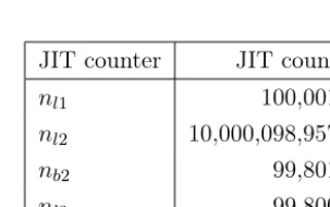
ℓ. Table1 and Table 2demonstrate this on the trace fragments of the nested loop example. The first two columns show the JIT counters, the remaining three columns show the frequency of the four trace fragments, and how they are derived from the counters. Note that not all counters reach the values one would expect from the loop bounds. This is because counting only starts once code has been compiled; iterations in warm-up phase of the JIT compiler are lost. The hotness threshold is currently 131 for loops.

JIT counter JIT count

nl1 100,001 nl2 10,000,098,957 nb2 99,801 nl3 99,800

Table 1

JIT counters and counts for program in Figure1.

3.3 JIT Instruction Classes

fragment frequency expression frequency l1 to l2 nl1 100,001

l2 to g2 nb2 99,801

l2 to j1 nl2−n_b2 9,999,999,156

l3 to j2 nl3 99,800

Table 2

JIT counters and trace fragment frequencies for program in Figure1.

other instructions; this is based on the idea that debug operations are removed by optimisations and do not count towards runtime execution costs.

It was further theorised that some instructions will be more costly than oth-ers. The set of all non-debug instructions was further subdivided into high-cost instructions high and low-cost instructions low, based on their expected relative performance.

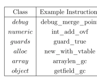
Class Example Instructions

debug debug_merge_point

numeric int_add_ovf

guards guard_true

alloc new_with_vtable

array arraylen_gc

object getfield_gc

Table 3

RPython JIT Instruction Classes

Further classification of the instructions can be made based on the conceptual grouping of them and makes no assumptions of their performance characteristics. The classes are object read and write instructionsobject, guardsguards, numerical instructions numeric, memory allocation instructions alloc and array instructions

array. These classes are described in Table3. Jump instructions are ignored, since there is only ever one in a trace. External calls are excluded as two foreign function calls could do radically different things.

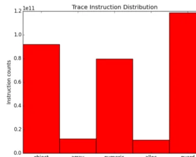
A histogram of JIT operations, taken from traces generated by all the cross-implementation benchmarks and shown in Figure3, shows that overall these traces are also dominated by instructions from the guards,objects and numericclasses.

4

JIT-based Cost Models

Fig. 3. Most common instructions in cross-implementation Pycket benchmarks

4.1 Trace Cost Models

We start with cost models for individual traces. Let Tr be an arbitrary trace of length n, that is, Tr = op1. . .op_n is a sequnce of instructions op_i. A trace cost

model γ is a function mapping Tr to itspredicted trace cost γ(Tr), whereγ(Tr) is a dimensionless number, (ideally) proportional to the time to execute Tr. Since the runtime of Trmay depend on the hardware architecture, the trace cost model may be specific to a particular architecture.

4.1.1 Null Cost Model (CM0)

The simplest possible trace cost model assigns the same cost to each trace, regardless of its length and the instructions contained. The purpose of this null cost model, which is formally defined by Equation (1), is to serve as a baseline to compare the accuracy of other cost models against. Using this model to calculate the cost for whole programs (Section 4.2) can be considered roughly equivalent to using a loop counting control-flow analysis for estimating the execution time of a program. Note that the null cost model is architecture independent.

γ(Tr) = 1 (1)

4.1.2 Counting Cost Model (CMC)

A slightly more sophisticated trace cost model declares the cost of a trace to be its length, counting the number of instructions (ignoring debug instructions, which are not executed at runtime). This counting cost model is defined by Equation (2) and is architecture independent.

γ(Tr) =

n

i=1

0, ifopi∈debug

4.1.3 Weighted Cost Model (CMW)

Certain types of instructions are likely to have greater execution time, for example memory accesses may be orders of magnitude slower than register accesses. A more intricate cost model can be obtained by applying a weighting factor to each of the instruction classes described in Section3.3. Equation (3) shows the definition of this

weighted cost model, parameterised by abstract weights a, b,c, dand e.

γ(Tr) =

n i=1 ⎧ ⎪ ⎪ ⎪ ⎪ ⎪ ⎪ ⎪ ⎪ ⎪ ⎨ ⎪ ⎪ ⎪ ⎪ ⎪ ⎪ ⎪ ⎪ ⎪ 

0, ifop_i ∈debug a, ifop_i ∈array b, ifop_i ∈numeric c, ifop_i ∈alloc d, ifop_i ∈guard e, ifop_i ∈object

(3)

The accuracy of the model depends on the concrete weights, and their choice depends on the actual architecture. Section4.3demonstrates how to obtain concrete weights for a reasonably accurate model.

4.2 Whole Program Cost Models

Let P be a program. During an execution of P, the JIT compiler generates m

distinct tracesTrj and massociated trace counters nj.

Given a (null, counting or weighted) trace cost model γ, we define the (null, counting or weighted) cost Γ(P) of P by summing up the cost of all traces, each weighted by their execution frequency; see Equation (4) for a formal definition.

Γ(P) =

m

j=1

njγ(Trj) (4)

Note thatΓis not apredictive cost model, as its definition relies on traces and trace counters, and the latter are only available after the execution of a program. However, Γ can still be useful for predicting the cost of transformations, as demonstrated in Section5.

4.3 Calibrating Weights for CMW

To use the abstract weighted cost modelCMW (Section4.1.3), it is necessary to find

concrete values for the weight parametersa, . . . , ein Equation (3). Ideally, program cost Γ(P) is proportional to program runtime t(P). That is, ideally there exists

k >0such that Equation (5) holds for all programs P.

Γ(P) =k t(P) (5)

4.3.1 Benchmarks

For the purpose of calibrating weights we use 41 programs from the standard Pycket benchmark suite pycket-bench [31] and the RacketProgramming Languages Bench-mark Game suite [18]. The programs used are a subset of the full suite, as programs that result in failing benchmark runs or which contain calls to foreign functions are omitted. Foreign function calls are removed as it is unlikely that any two foreign function calls are doing the same thing or take the same time.

For each program, we record the execution time, averaging over 10 runs. We also record all traces and the values of all trace counters; since all benchmarks are deterministic traces and trace counters do not vary between runs.

The Pycket version used for these experiments is revision e56ba66d71 of the

trace-analysis branch of our custom fork [29], built with Racket version 6.1 and revision 79009 of the RPython toolchain. The experiments are run on a 16 core 2.0 GHz Xeon server with 64 GB of RAM running Ubuntu 14.04.

4.3.2 Linear Regression

Picking an arbitrary value for k, e.g. k = 1, we derive the following relation from Equations (5) and (4).

t(Pl) = Γ(Pl) +ǫl= ml

j=1

nljγ(Trlj) +ǫl (6)

Pl is thelth benchmark program, generating mltraces Trlj and trace countersnlj, t(Pl) is the observed average runtime of Pl, and ǫl is the error term. Equation (6)

becomes a model for linear regression by expanding γ according to its definition (3), which turns the right-hand side into an expression linear in the five unknown weights a, . . . , e.

Weights are implicitly constrained to be non-negative, as negative weights would suggest that corresponding instructions take negative time to execute, which is phys-ically impossible. To honour the non-negativity constraint, weights are estimated by non-negative least squares linear regression.

γ(Tr) =

k i=1 ⎧ ⎪ ⎪ ⎪ ⎪ ⎨ ⎪ ⎪ ⎪ ⎪ 

4.884×10−4, if op

i∈numeric

4.797×10−3, if op

i∈alloc

4.623×10−4, if op

i∈guard

0, otherwise

(7)

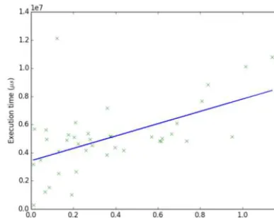
Equation (7) shows the resulting weighted cost model for the Xeon server architec-ture. This model only attributes non-zero cost to allocation, numeric instructions and guards, implying that object and array access instructions have negligible cost. The regression fit for this cost model is shown in Figure 4. The fit is obviously linear but rather coarse, indicating thatCMW is not a very accurate model. There is

Fig. 4. Execution time vs cost forCMW determined using linear regression

rather than compiled code, resulting in an underestimation of cost due to lack of trace output to measure. We note that linear regression fits forCMC and CM0 are

visibly worse than the fit forCMW, which implies that their accuracy is lower than CMW.

5

Costing Transformations

The main purpose of a cost model in the AJITPar project is to enable the selec-tion and parameterisaselec-tion of appropriate dynamic transformaselec-tions. This secselec-tion identifies the transforms and explores how accurately the cost models predict the execution time of programs before and after transformation.

5.1 Skeleton Transforms

In AJITPar parallel programs are expressed by composingalgorithmic skeletons[17] from an Adaptive Skeletons (AS) library [27].

Adaptive skeletons are based on a standard set of algorithmic skeletons for spec-ifying task-based parallelism within Racket. The AS framework expands skeletons to task graphs and schedules tasks to workers; expansion and scheduling happen at runtime to support tasks with irregular granularity. The AS framework piggy-backs on Pycket to analyze the cost of tasks as they are executed. The cost information is used both to guide the dynamic task scheduler as well as a skeleton transfor-mation engine. The latter adapts the task granularity of the running program to suit the current architecture by rewriting skeletons according to a standard set of equations [27].

−− map s k e l e t o n s

parMap : : ( a → b ) → [ a ] → [ b ]

parMap f [ ] = [ ]

parMap f ( x : xs ) = spawn f x : parMap f xs

parMapChunk : : I n t → _{( a} → _{b )} → _{[ a ]} → _{[ b ]}

parMapChunk k f xs = concat $ parMap (map f ) $ chunk k xs

parMapStride : : I n t → _{( a} → _{b )} → _{[ a ]} → _{[ b ]}

parMapStride k f xs = concat $ transpose $ parMap (map f ) $ transpose $ chunk k xs

−− d i v i d e and c onq u e r s k e l e t o n s

parDivconq : : ( a → [ a ] ) → ( [ b ] → b ) → ( a → b ) → a → b

parDivconq d i v comb conq x = c a s e d i v x o f

[ ] → spawn conq x

ys → spawn comb (map (parDivconq d i v comb conq ) ys )

parDivconqThresh : : ( a → Bool ) → ( a → [ a ] ) → ( [ b ] → b ) → ( a → b ) → a → b

parDivconqThresh t h r e s h d i v comb conq x = i f t h r e s h x

then spawn (divconq d i v comb conq ) x e l s e c a s e d i v x o f

[ ] → spawn conq x

ys → comb (map (parDivconqThresh p d i v comb conq ) ys )

−− s i g n a t u r e s o f a u x i l i a r y f u n c t i o n s

chunk : : I n t → [ a ] → [ [ a ] ]

map : : ( a → _{b )} → _{[ a ]} → _{[ b ]}

concat : : [ [ a ] ] → [ a ]

divconq : : ( a → _{[ a ] )} → _{( [ b ]} → _{b )} → _{( a} → _{b )} → _a → _b

transpose : : [ [ a ] ] → [ [ a ] ]

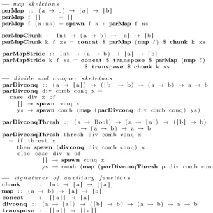
Fig. 5. AJITPar base skeletons and tunable skeletons.

parDivconqThresh, are shown in Figure5, specified in a Haskell-style pseudocode5

. Code which uses these skeletons can be transformed by modifying the first argument which serves as a tuning parameter; we will useτ to denote this tuning parameter. The AJITPar system aims to transform skeletons such that the resulting tasks are of optimal granularity, i.e. execute for about 10 to 100 milliseconds on average. To this end, the system monitors the runtime of tasks and computes their cost as they complete, following Equation (4). If the system sees too many tasks fall outwith the optimal granularity range, it will attempt to transform the skeleton that generated the tasks. In the simplest case this is done by changing the tuning parameter τ as follows.

Let t0 and γ0 be the observed average runtime and cost of tasks generated by

the skeleton’s current tuning parameter τ0. The system computes k = t0/γ0 and

picks a target granularityt1(in the range 10 to 100 milliseconds) and corresponding

target cost γ1 = t1/k. Then the system picks the new tuning parameter τ1 such

that the cost ratio γ1/γ0 and the tuning ratio τ1/τ0 are related by the skeleton’s

cost derivative.

The cost derivative is a function expressing the change of cost γ in response

5

Benchmark Input Skeleton(s) Matrix multiplication 1000x1000 matrices parMapChunk

SumEuler [1...4000] parMapChunk; parMapStride Fibonacci 42 parDivconqThresh

k-means sample data parMapChunk Mandelbrot 6000x6000 parMapChunk

Table 4

Benchmarks with their input and applied skeletons

to the change of the tuning parameter τ. For example, the cost derivative for the

parMapChunk skeleton is the constant function 1 because doubling the chunk size τ

doubles the cost of tasks. In contrast, the derivative forparMapStride is the function

1/x because doubling the stride width τ halves the cost of individual tasks. Note that in general, the cost derivative is specific to the skeleton but independent of benchmark application and architecture.

Underlying this method of tuning τ is the assumption that the time/cost ratio

k is independent of τ. In the rest of this section, we will empirically demonstrate that this is indeed the case as long as task granularity is not too small.

5.2 Experiments

The suitability of the cost models for predicting the effect of applying transforms on execution time is evaluated. A cost model will be considered sufficiently accurate if the ratio k of execution time to predicted cost is constant across differentτ values for each program.

5.2.1 Benchmarks and transforms

The benchmarks used in these experiments are shown in Table 4, and the sources of the benchmarks are available at [30]. For most benchmarks it is obvious what tasks compute, e.g. in the case of matrix multiplication a chunk of rows of the result matrix. k-means is a special case, its tasks do not compute a clustering but classify a chunk of the input data according to the current centroids; this is the parallel part of each iteration of the standard cluster refinement algorithm. The input data for k-means consists of 1024000 data points of dimension 1024, to be grouped into 5 clusters. The experiments are carried out on the same hardware and software platforms as in Section4.3.1.

5.2.2 Experimental Design

difference in trace counters between the two runs accurately reflects to the trace counters of the task6

.

Mandelbrot and SumEuler areirregular benchmarks, that is, work is distributed non-uniformly, making some tasks harder than others. To investigate the accuracy of the cost model in the presence of irregular parallelism, we repeat the Mandelbrot and chunked SumEuler experiments with different chunks.

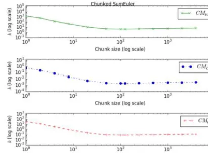
5.2.3 Results

The graphs of time/cost ratio k against tunable paramater τ for each benchmark and cost model can be found in Figures6to11. The rightmost point on each graph represents theτ equivalent to one worker, and thus the untransformed version of that code; moving rightwards along the x-axis corresponds to increasingly coarse-grained tasks.

Figure12shows the plot of k (for cost modelCMW) againstτ for each of three

different chunks of Mandelbrot, showing how irregularity affects the prediction. Ta-ble5shows the stable values of time/cost ratiokto which the benchmarks converge; the table also shows the range of values thatkcan take and a “minimum” task gran-ularity (Section 5.3).

Fig. 6.kvsτ for Matrix multiplication benchmark

5.3 Discussion

The overall shape of graphs in Figures 6 to 11is the same for all benchmarks and cost models: The time/cost ratio k starts out high (on the left) and falls at first as task granularity increases, then stabilises. The value of k the graphs stabilise at depends on the benchmark and on the cost model; forCMW the stablekvalues are

listed in Table 5. By design of CMW these values cluster around 1 though none of

them is particularly close to 1, indicating that CMW is not particularly accurate

for any of the benchmarks, over- or under-estimating the actual execution time by

6

Fig. 7.kvsτ for irregular chunked SumEuler benchmark

Fig. 8. kvsτ for strided SumEuler benchmark

Fig. 9. kvsτ for Fibonacci benchmark

a factor of2to7. This is expected given the coarseness of the fit ofCMW shown in

the previous section (Figure 4).

gran-Fig. 10.kvsτ for k-means benchmark

Fig. 11. kvsτ for Mandelbrot benchmark

Fig. 12.kvsτ for Mandelbrot benchmark (CMW) comparing 3 chunks

Benchmark stablek range ofk min. task granularity for stablek

Matrix Multiplication 0.579 0.201 <11400μs

Strided SumEuler 6.87 1450 306μs

Chunked SumEuler 4.31 1460 129μs

Fibonacci 0.542 1.55 294μs

k-means 0.535 0.847 <12100μs

Mandelbrot 0.251 0.0187 <117000 μs

Table 5

Stablekvalues for each benchmark (cost modelCMW)

granularity crosses a certain threshold, around 100 to 300 μs as listed in Table 5, the value ofkstabilises. This suggests that the cost models are particularly inaccu-rate for small tasks, possibly due to the fact that smaller tasks run through fewer traces, but do become more accurate as task size increases. In particular, the cost models are reasonably accurate for tasks in the target granularity range of 10 to 100 milliseconds.

For matrix multiplication and Mandelbrot the range of k listed in Table 5 is small. For k-means the range would also be small (around0.3) if the unusually high

k for the smallest task granularity were disregarded as an outlier.7

This correlates with minimum task granularities that are quite high (10 to 120 milliseconds); in fact, these granularities are already in the target range. Thus, for these benchmarks the cost models are reasonably accurate over the whole range of the tuning parameterτ. Another source of inaccuracy for cost prediction, besides ultra-low task granular-ity, is irregularity. The chunked SumEuler and Mandelbrot benchmarks do exhibit irregular parallelism. In the case of SumEuler, chunks at the lower end of the in-terval give rise to smaller tasks than chunks at the upper end, and in the case of Mandelbrot, chunks at the top and bottom of the image produce smaller tasks than chunks in the middle. The graphs in Figures7and 11show plots of kfor chunks in the middle of the interval or image rather than the average over all chunks, in an attempt to account for the effect of irregularity. Figure 12contrasts the time/cost ratiokof a chunk at the top of the image (Chunk 0) with two chunks in the middle. Thek for Chunk 0 is markedly different from the other two and not stable, though the graphs do converge as granularity increases, which correlates with the fact that irregularity decreases as chunk size increases. We note that while the moderate ir-regularity of Mandelbrot causes some loss of accuracy, it is not too bad: the ratio between the most extremekof Chunk 0 and the stable value ofk for Mandelbrot is less than a factor of 3. In contrast, the ratio between task runtimes for Chunk 0 and average task runtimes for Mandelbrot is a factor of more than 10. Thus, the cost models are somewhat able to smooth the inaccuracies in prediction that are caused by irregular task sizes.

Finally, on the evidence presented here, it does look like all three cost models are

7

equally well suited to predicting the cost of transformations. While this is the case for simple transformations that only change the value of a single tuning parameter

τ, this need no longer be the case when trying to cost a chain of two transformations. In future work, we aim to systematically predict the cost of chains of transformations of skeleton expressions comprising multiple skeletons, e.g. a parallel map followed by a parallel reduce. We expect that in these cases there will be a bigger difference between the set of traces pre- and post-transformation than what we currently see. Hence we expect the actual content of the traces to matter more, and cost model

CMW to beat the other two on accuracy of prediction.

6

Discussion and Ongoing work

We have designed and implemented a system for extracting JIT trace information from the Pycket JIT compiler (Section 3). We have defined three lightweight cost models for JIT traces, ranging from the extremely simple loop counting modelCM0

to the relatively simple instruction counting modelCMC to the architecture-specific

weighted model CMW. To automatically determine appropriate weights for CMW

we have run a linear regression over the Pycket benchmark suite (Section 4). We have used all three cost models to compare the relative cost of tasks generated by six skeleton-based benchmarks pre- and post-transformation, where the skeleton transformations are induced by changing a skeleton-specific tuning parameter. We have found that the effect of these transformations on task runtime can be predicted accurately using our cost models, once the task granularity rises above a threshold (Section 5).

We have demonstrated that even the simplest, architecture-independent cost model described in this paper allows us to accurately predict the effect of simple transformations on task runtime. We expect that the architecture-specific model

CMW will be more accurate when predicting the task runtime of more complex

transformations, e.g. chains of transformations (as arise naturally when transform-ing complex skeleton expressions by rewrittransform-ing). We further speculate that similar techniques can be used to identify lightweight cost models based on the traces pro-duced by the JIT compilers for other languages, e.g. Python, Javascript, etc.

In future work, the AJITPar project plans to use cost model CMW in its efforts

to adapt task granularity to best suit the underlying parallel architecture. More precisely, CMW will be used to tune skeleton parameters (as outlined in Section 5)

and also to select the most promising candidate expressions for skeleton rewriting. The AJITPar project plans to evaluate whether this cost-model based adaptive framework does deliver portable parallel performance by benchmarking several case studies on multiple architectures, ranging from multicore desktops to clusters of servers with several hundred cores.

References

(ECRTS), 2014 26th Euromicro Conference on, pages 266–275. IEEE, 2014.

[2] AJITPar project.http://www.dcs.gla.ac.uk/~pmaier/AJITPar/, 2014. Accessed: 2014-11-13.

[3] Elvira Albert, Puri Arenas, Jesús Correas, Samir Genaim, Miguel Gómez-Zamalloa, Enrique Martin-Martin, Germán Puebla, and Guillermo Román-Díez. Resource analysis: From sequential to concurrent and distributed programs. FM 2015: Formal Methods, pages 3–17, 2015.

[4] Elvira Albert, Puri Arenas, Samir Genaim, German Puebla, and Damiano Zanardini. Cost analysis of object-oriented bytecode programs. Theoretical Computer Science, 413(1):142–159, 2012.

[5] Elvira Albert, Jesús Correas, Germán Puebla, and Guillermo Román-Díez. Incremental resource usage analysis. In Proceedings of the ACM SIGPLAN 2012 workshop on Partial evaluation and program manipulation, pages 25–34. ACM, 2012.

[6] David Aspinall, Robert Atkey, Kenneth MacKenzie, and Donald Sannella. Symbolic and analytic techniques for resource analysis of Java bytecode. In Trustworthly Global Computing, pages 1–22. Springer, 2010.

[7] Marco Autili, Paolo Di Benedetto, and Paola Inverardi. A hybrid approach for resource-based comparison of adaptable Java applications. Science of Computer Programming, 78(8):987–1009, 2013. [8] John Aycock. A brief history of just-in-time.ACM Computing Surveys (CSUR), 35(2):97–113, 2003. [9] Gilles Barthe, Pierre Crégut, Benjamin Grégoire, Thomas Jensen, and David Pichardie. The MOBIUS

proof carrying code infrastructure. In Formal Methods for Components and Objects, pages 1–24. Springer, 2008.

[10] Spenser Bauman, Carl Friedrich Bolz, Robert Hirschfeld, Vasily Krilichev, Tobias Pape, Jeremy G. Siek, and Sam Tobin-Hochstadt. Pycket: A tracing JIT for a functional language. InICFP ’15, 2015. To appear.

[11] Carl Friedrich Bolz, Antonio Cuni, Maciej Fijalkowski, and Armin Rigo. Tracing the meta-level: PyPy’s tracing JIT compiler. InProceedings of the 4th workshop on the Implementation, Compilation, Optimization of Object-Oriented Languages and Programming Systems, pages 18–25. ACM, 2009. [12] Carl Friedrich Bolz, Adrian Kuhn, Adrian Lienhard, Nicholas D Matsakis, Oscar Nierstrasz, Lukas

Renggli, Armin Rigo, and Toon Verwaest. Back to the future in one week - implementing a Smalltalk VM in PyPy. InSelf-Sustaining Systems, pages 123–139. Springer, 2008.

[13] Carl Friedrich Bolz, Tobias Pape, Jeremy Siek, and Sam Tobin-Hochstadt. Meta-tracing makes a fast Racket. 2014.

[14] István Bozó, Viktoria Fordós, Zoltán Horvath, Melinda Tóth, Dániel Horpácsi, Tamás Kozsik, Judit Köszegi, Adam Barwell, Christopher Brown, and Kevin Hammond. Discovering parallel pattern candidates in Erlang. InProceedings of the Thirteenth ACM SIGPLAN workshop on Erlang, pages 13–23. ACM, 2014.

[15] Carlo Brandolese, William Fornaciari, Fabio Salice, and Donatella Sciuto. Source-level execution time estimation of C programs. InProceedings of the ninth international symposium on Hardware/software codesign, pages 98–103. ACM, 2001.

[16] Christopher Brown, Marco Danelutto, Kevin Hammond, Peter Kilpatrick, and Archibald Elliott. Cost-directed refactoring for parallel Erlang programs. International Journal of Parallel Programming, 42(4):564–582, 2014.

[17] Murray I Cole.Algorithmic skeletons: structured management of parallel computation. Pitman London, 1989.

[18] Computer languages benchmark game.http://benchmarksgame.alioth.debian.org/. Accessed: 2016-01-09.

[19] Ugo Dal Lago and Ricardo Peña. Foundational and Practical Aspects of Resource Analysis: Third International Workshop, FOPARA 2013, Bertinoro, Italy, August 29-31, 2013, Revised Selected Papers, volume 8552. Springer, 2014.

[20] Christian Ferdinand and Reinhold Heckmann. aiT: Worst-case execution time prediction by static program analysis. InBuilding the Information Society, pages 377–383. Springer, 2004.

[21] Khronos OpenCL Working Group et al. The OpenCL specification.version, 1(29):8, 2008.

[22] Shuai Hao, Ding Li, William GJ Halfond, and Ramesh Govindan. Estimating mobile application energy consumption using program analysis. InSoftware Engineering (ICSE), 2013 35th International Conference on, pages 92–101. IEEE, 2013.

[24] Simon L Peyton Jones. Compiling Haskell by program transformation: A report from the trenches. In

Programming Languages and Systems - ESOP’96, pages 18–44. Springer, 1996.

[25] Simon Peyton Jones, Andrew Tolmach, and Tony Hoare. Playing by the rules: rewriting as a practical optimisation technique in GHC. InHaskell workshop, volume 1, pages 203–233, 2001.

[26] Rody WJ Kersten, Bernard E Gastel, Olha Shkaravska, Manuel Montenegro, and Marko CJD Eekelen. ResAna: a resource analysis toolset for (real-time) JAVA.Concurrency and Computation: Practice and Experience, 26(14):2432–2455, 2014.

[27] Patrick Maier, John Magnus Morton, and Phil Trinder. Towards an adaptive framework for performance portability. InPre-proceedings of IFL 2015, Koblenz, Germany, 2015.

[28] Patrick Maier, Rob Stewart, and Philip W Trinder. Reliable scalable symbolic computation: The design of SymGridPar2.Computer Languages, Systems & Structures, 40(1):19–35, 2014.

[29] John Magnus Morton. Pycket fork. https://github.com/magnusmorton/pycket. Accessed: 2016-01-09.

[30] John Magnus Morton. Trace analysis utilities. https://github.com/magnusmorton/trace-analysis. Accessed 2016-01-09.

[31] Tobias Pape. Benchmarking pycket against some Schemes. https://github.com/krono/pycket-bench. Accessed: 2016-01-09.

[32] Pypy. http://pypy.org. Accessed 2015-03.

[33] Python.http://python.org. Accessed 2015-03.

[34] Vítor Rodrigues, Benny Akesson, Mário Florido, Simão Melo de Sousa, João Pedro Pedroso, and Pedro Vasconcelos. Certifying execution time in multicores.Science of Computer Programming, 111:505–534, 2015.

[35] Norman Scaife, Susumi Horiguchi, Greg Michaelson, and Paul Bristow. A parallel SML compiler based on algorithmic skeletons.Journal of Functional Programming, 15(04):615–650, 2005.

[36] Daniel Spoonhower, Guy E Blelloch, Robert Harper, and Phillip B Gibbons. Space profiling for parallel functional programs. ACM Sigplan Notices, 43(9):253–264, 2008.

[37] Guy Lewis Steele Jr and Gerald Jay Sussman. The revised report on SCHEME: A dialect of LISP. Technical report, DTIC Document, 1978.

[38] Timing analyis on code-level (TACLe). http://www.tacle.eu. Accessed: 2016-1-11.

[39] Topaz. https://github.com/topazproject/topaz. Accessed: 2015-03.

[40] Philip W Trinder, Murray I Cole, Kevin Hammond, H-W Loidl, and Greg J Michaelson. Resource analyses for parallel and distributed coordination. Concurrency and Computation: Practice and Experience, 25(3):309–348, 2013.