Synchronous Tree Adjoining Machine Translation

Synchronous Tree Adjoining Machine Translation

Steve DeNeefe and Kevin Knight USC Information Sciences Institute 4676 Admiralty Way, Suite 1001

Marina del Rey, CA 90292 USA

{sdeneefe,knight}@isi.edu

Abstract

Tree Adjoining Grammars have well-known advantages, but are typically considered too difficult for practical systems. We demon-strate that, when done right, adjoining im-proves translation quality without becoming computationally intractable. Using adjoining to model optionality allows general translation patterns to be learned without the clutter of endless variations of optional material. The appropriate modifiers can later be spliced in as needed.

In this paper, we describe a novel method for learning a type of Synchronous Tree Ad-joining Grammar and associated probabilities from aligned tree/string training data. We in-troduce a method of converting these gram-mars to a weakly equivalent tree transducer for decoding. Finally, we show that adjoining results in an end-to-end improvement of +0.8 BLEUover a baseline statistical syntax-based MT model on a large-scale Arabic/English MT task.

1 Introduction

Statistical MT has changed a lot in recent years. We have seen quick progress from manually crafted linguistic models to empirically learned statistical models, from word-based models to phrase-based models, and from string-based mod-els to tree-based modmod-els. Recently there is a swing back to incorporating more linguistic information again, but this time linguistic insight carefully guides the setup of empirically learned models.

Shieber (2007) recently argued that proba-bilistic Synchronous Tree Adjoining Grammars (Shieber and Schabes, 1990) have the right com-bination of properties that satisfy both linguists and empirical MT practitioners. So far, though, most work in this area has been either more lin-guistic than statistical (Abeille et al., 1990) or statistically-based, but linguistically light (Nesson et al., 2006).

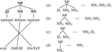
Current tree-based models that integrate lin-guistics and statistics, such as GHKM (Galley et al., 2004), are not able to generalize well from a single phrase pair. For example, from the data in Figure 1, GHKM can learn rule (a) to translate nouns with two pre-modifiers, but does not gener-alize to learn translation rules (b) - (d) without the optional adjective or noun modifiers. Likewise, none of these rules allow extra material to be intro-duced, e.g. “Pakistan’s national defense minister”. In large enough training data sets, we see many examples of all the common patterns, but the rarer patterns have sparse statistics or poor coverage.

NP

JJ

national

NN

defense

NN

minister

wzyr AldfAE AlwTnY

(a) NP

JJ1NN2NN3

↔ NN3NN2JJ1

(b) NP

NN1NN2

↔ NN2NN1

(c) NP

JJ1NN2

↔ NN2JJ1

(d) NP NN1

↔ NN1

Figure 1: Rule (a) can be learned from this training example. Arguably, the more general rules (b) -(d) should also be learnable.

To mitigate this problem, the parse trees used as training data for these systems can be binarized (Wang et al., 2007). Binarization allows rules with partial constituents to be learned, resulting in more general rules, richer statistics, and better phrasal coverage (DeNeefe et al., 2007), but no principled required vs. optional decision has been made. This method’s key weakness is that binarization always keeps adjacent siblings together, so there is no way to group the head with a required complement if optional information intervenes between the two. Furthermore, if all kinds of children are consid-ered equally optional, then we have removed im-portant syntactic constraints, which may end up permitting too much freedom. In addition, spu-rious alignments may limit the binarization

nique’s effectiveness.

In this paper, we present a method of learning a type of probabilistic Synchronous Tree Adjoin-ing Grammar (STAG) automatically from a cor-pus of word-aligned tree/string pairs. To learn this grammar we use linguistic resources to make the required vs. optional decision. We then directly model the optionality in the translation rules by learning statistics for the required parts of the rule independently from the optional parts. We also present a method of converting these rules into a well-studied tree transducer formalism for decod-ing purposes. We then show that modeldecod-ing option-ality using adjoining results in a statistically sig-nificant BLEUgain over our baseline syntax-based model with no adjoining.

2 Translation Model

2.1 Synchronous Tree Insertion Grammars

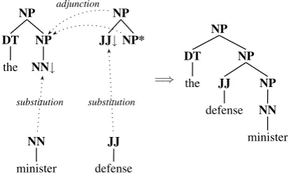
Tree Adjoining Grammars (TAG), introduced by Joshi et al. (1975) and Joshi (1985), allow inser-tion of unbounded amounts of material into the structure of an existing tree using an adjunction operation. Usually they also include a substitution operation, which has a ‘fill in the blank’ seman-tics, replacing a substitution leaf node with a tree. Figure 2 visually demonstrates TAG operations. Shieber and Schabes (1990) offer a synchronous version of TAG (STAG), allowing the construc-tion of a pair of trees in lockstep fashion using the TAG operations of substitution and adjunction on tree pairs. To facilitate this synchronous behav-ior, links between pairs of nodes in each tree pair define the possible sites for substitution and ad-junction to happen. One application of STAG is machine translation (Abeille et al., 1990).

One negative aspect of TAG is the compu-tational complexity: O(n6) time is required for monolingual parsing (and thus decoding), and STAG requires O(n12) for bilingual parsing (which might be used for training the model di-rectly on bilingual data). Tree Insertion Grammars (TIG) are a restricted form of TAG that was in-troduced (Schabes and Waters, 1995) to keep the same benefits as TAG (adjoining of unbounded material) without the computational complexity— TIG parsing isO(n3). This reduction is due to a limitation on adjoining: auxiliary trees can only introduce tree material to the left or the right of the node adjoined to. Thus an auxiliary tree can be classified by direction as left or right adjoining.

adjunction

NP

DT

the

NP

NN↓

NP

JJ↓NP*

substitution substitution

NN

minister

JJ

defense

=⇒

NP

DT

the

NP

JJ

defense

NP

NN

minister

Figure 2: TAG grammars use substitution and ad-junction operations to construct trees. Substitu-tion replaces the substituSubstitu-tion node (marked with

↓) with another tree. Adjunction inserts an aux-iliary tree—a special kind of tree fragment with a foot node (marked with *)—into an existing tree at a permitted non-terminal node. Note that in TAG, adjunctions are permitted atanynon-terminal with the same label as the root and foot node of the auxiliary tree, while in STAG adjunctions are re-stricted to linked sites.

Nesson et al. (2006) introduce a probabilis-tic, synchronous variant of TIG and demonstrate its use for machine translation, showing results that beat both word-based and phrase-based MT models on a limited-vocabulary, small-scale train-ing and test set. Training the model uses an

O(n6_{) bilingual parsing algorithm, and decoding} isO(n3). Though this model uses trees in the for-mal sense, it does not create Penn Treebank (Mar-cus et al., 1993) style linguistic trees, but uses only one non-terminal label (X) to create those trees us-ing six simple rule structures.

The grammars we use in this paper share some properties in common with those of Nesson et al. (2006) in that they are of the probabilistic, syn-chronous tree-insertion variety. All pairs of sites (both adjunction and substitution in our case) are explicitly linked. Adjunction sites are restricted by direction: at each linked site, the source and target side each specify one allowed direction. The re-sult is that each synchronous adjunction site can be classified into one of four direction classes: {LR, LL, RR, RL}. For example, LR means the source side site only allows left adjoining trees and the target side site only allows right adjoining trees.

There are several important differences between our grammars and the ones of Nesson et al. (2006):

Penn Treebank-style linguistic tree on the En-glish (target) side, and a hierarchical structure using only a single non-terminal symbol (X) on the source side. We believe this provides the rich information needed in the target lan-guage without over-constraining the model.

Substitution Sites/Non-lexical trees: We use both substitution and adjunction (Nesson et al. (2006) only used adjunction) and do not require all trees to contain lexical items as is commonly done in TIG (Schabes and Waters, 1995).

Single Adjunction/Multiple Sites: Each non-terminal node in a tree may allow multiple adjunction sites, but every site only allows at most one adjunction,1a common assumption for TAG as specified in the Vijay-Shanker (1987) definition.

Here are some examples of automatically learned translation rules with interpretations of how they work:

1. simple lexical rules for translating words or phrases:

IN

without

⇐⇒ X

AlA

interpretation: translate the Arabic word “AlA” as the preposition “without”

2. rules with substitution for translating phrases with holes (substitution sites are designated by an arrow and numeric subscript, e.g.

NP↓₁):

PP

PP

IN

of

NP↓₁

⇐⇒ X

X↓₁

interpretation: insert “of” to turn a noun phrase into a prepositional phrase

3. simple adjoining rules for inserting optional modifiers (adjoining sites are designated by

1_{An adjoined rule may itself have adjoining sites allowing}

further adjunction.

an alphabetic subscript beforeorafter a non-terminal to indicate direction of adjoining, e.g._aNP):

aNP

JJ↓₁ NP*

⇐⇒

X

X* X_a

X↓₁

interpretation: adjoin an adjective before a noun in English but after in Arabic, and al-lowing further adjoinings in those same di-rections afterward

4. rules with multiple adjunction and substitu-tion sites:

aS

NP↓1 bSc

VPd

VPe

VBD↓2

NP↓3

⇐⇒

X

aX

X↓2

X

X↓1 e,bXd,c

X↓3

interpretation: translate an Arabic sentence in VSO form into an English sentence in SVO form, with multiple adjoining options

2.2 Generative Story

When we use these rules to translate from a for-eign sentence f into an English sentence e, we use several models together in a log-linear fash-ion, but our primary model is a joint model of

P(etree, ftree), which is our surrogate for directly

modeling P(e|f). This can be justified because

P(e|f) = P_P(₍e,f_f)), and P(f) is fixed for a given foreign sentence. Therefore:

argmax

e P(e|f) = argmaxe P(e, f)

≈ yield(argmax

etree P(etree, ftree))

≈ yield(argmax

etree P(detree,ftree))

where d_etree,ftree is a derivation tree of rules that generates e_tree andf_tree. In other words, e, the highest probability translation off, can be approx-imated by taking the yield of the highest proba-bility tree e_tree that is a translation of the high-est probability tree off. This can further be ap-proximated by the highest probability derivation of rules translating betweenf andevia trees.

Now we define the probability of generating

representing a rule with a single substitution site,2

&TOP↓, X↓', a tree pair can be generated by the following steps:

1. For each substitution sites_iin the current rule

r1:

(a) Choose with probability

Psub(r2|&labelL(si),labelR(si)') a rule r2 having root node labels labelL(si)

and label_R(s_i) that match the left and right labels ats_i.

2. For each adjunction site s_i,r1 in the current ruler₁:

(a) Choose with rule-specific probability

Pifadj(decisionadjoin|si,r1, r1) choose whether or not to adjoin at the current sites_i,r1.

(b) If we are adjoining at site

si,r1, choose with probability Padj(r2|d,&labelL(si,r1),labelR(si,r1)')

a rule r₂ of direction class d having root node labels label_L(s_i,r1) and label_R(s_i,r1) that match the left and right labels ats_i,r1.

3. Recursively process each of the added rules

For all substitution rulesr_s, adjoining rulesr_a, and adjoining sitess_i,r, the probability of a deriva-tion tree using these rules is the product of all the probabilities used in this process, i.e.:

Pderiv =

!

rs

"

Psub(rs|&rootL(rs),rootR(rs)')·

!

si,rs

Pifadj(decisionadjoin|si,rs, rs)

#

·

!

ra

"

Padj(ra|dir(ra),&rootL(ra),rootR(ra)')·

!

si,ra

Pifadj(decisionadjoin|si,ra, ra)

#

Note that while every new substitution site re-quires an additional rule to be added, adjunction sites may or may not introduce an additional rule based on the rule-specific Pif_adj probability. This allows adjunction to represent linguistic optional-ity.

2_{Here and in the following, we usesiteas shorthand for}

synchronous site pair.

3 Learning the Model

Instead of using bilingual parsing to directly train our model from strings as done by Nesson et al. (2006), we follow the method of Galley et al. (2004) by dividing the training process into steps. First, we word align the parallel sentences and parse the English (target) side. Then, we transform the aligned tree/string training data into derivation trees of minimal translation rules (Section 3.1). Fi-nally, we learn our probability modelsP_sub,Pif_adj, andP_adj by collecting counts over the derivation trees (Section 3.2). This method is quick enough to allow us to scale our learning process to large-scale data sets.

3.1 Generating Derivation Trees and Rules

There are four steps in transforming the training data into derivation trees and rules, the first two operating only on the English parse tree itself:3

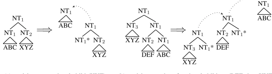
A. Marking Required vs. Optional. For each constituent in the English parse tree, we mark chil-dren as (H)ead, (R)equired, or (O)ptional elements (see step (a) in Figure 3). The choice of head, re-quired, or optional has a large impact on the gen-erality and applicability of our grammar. If all children are considered required, the result is the same as the GHKM rules of Galley et al. (2004) and has the same problem—lots of low count, syntactically over-constrained rules. Too many optional children, on the other hand, allows un-grammatical output. Our proposed model is a lin-guistically motivated middle ground: we consider the linguistic heads and complements selected by Collins’ (2003) rules to be required and all other children to be optional.

B. Parse tree to TIG tree. Next, we re-structure the English tree to form a TIG deriva-tion where head and required elements are substi-tutions, and optional elements are adjunctions (see step (b) in Figure 3). To allow for adjoining be-tween siblings under a constituent, we first do a head-out binarization of the tree. This is followed by excising4 any children marked as optional and replacing them with an adjunction site, as shown in Figure 4. Note that we excise a chain of op-tional children as one site with each opop-tional child

3_{Thesefirst two steps were inspired by the method Chiang}

(2003) used to automatically extract a TIG from an English parse tree.

4_{Excising is the opposite of adjoining: extracting out an}

S

ADVP , NP VP . ₌(a)_⇒

S

ADVP_O ,_O NP_R VP_H ._{O =}(b)_⇒

S

ADVP , NP VP .

Figure 3: Parse tree to TIG transformation: (a) mark constituent children with (H)ead, (R)equired, and (O)ptional, then (b) restructure the tree so that head and required elements are substitutions, while op-tional elements are adjoined (shown with dotted lines).

NT₁

NT₁

ABC NT₂

XYZ

=

⇒

NT₁

ABC NT₁

NT₁* NT₂

XYZ

NT₁

NT₃

XYZ

NT₁

NT₂

DEF NT₁

ABC

=

⇒

NT₁

NT₁

NT₁

NT₃

XYZ NT₁*

NT₂

DEF NT₁*

ABC

(a) excising one optional child (XYZ) (b) excising a series of optional children (DEF, then XYZ)

Figure 4: Two examples of excising auxiliary trees from a head-out binarized parse tree: (a) excising one optional left branch, (b) excising a chain of optional branches in the same (right) direction into a series of adjunctions. In both examples, the ‘ABC’ child is the head, while the other children are optional.

adjoined to the previous child, as in Figure 4(b).

C. Extracting rules and derivation trees. We now have a TIG derivation tree, with each elemen-tary tree attached to its parent by a substitution or adjunction link. We can now extract synchronous rules allowed by the alignments and syntactic con-stituents. This can be done using a method in-spired by the rule-extraction approach of Galley et al. (2004), but instead of directly operating on the parse tree we process the English TIG derivation tree. In bottom-up fashion, we visit each elemen-tary tree in the derivation, allowing a rule rooted at this tree to be extracted if its words or those of its descendants are aligned such that they are the English side of a self-contained parallel phrase (i.e., the foreign text of this phrase is not aligned to English leaves outside of the set of descendants). Otherwise, this elementary tree is rejoined with its parent to form a larger elementary tree. At the end of this process we have a new set of linked ele-mentary trees which make up the English side of the grammar, where each substitution or adjunc-tion link becomes a substituadjunc-tion or adjuncadjunc-tion site in the synchronous grammar.

On the foreign side we start with the foreign text of the self-contained parallel phrase and replace any parts of this phrase covered by substituted or

adjoined children of the English side tree with sub-stitution sites or adjunction site markers. From this, we produce a tree with a simple, regular form by placing all items under a root node labeled X. In the case of more than one foreign word or sub-stitution site, we introduce an intermediate level of X-labeled non-terminals to allow for possible ad-junction between elements, otherwise the adjoin-ing sites attach to the sadjoin-ingle root node. We attach all foreign-side adjoining sites to be left adjoining, except on the right side of the right-hand child.

It is possible to have the head child tree on the English side not aligned to anything, while the ad-joined children are. This may lead to rules with no foreign non-terminal from which to anchor the ad-junctions, so in this case, we attach adjoined child elementary trees starting from the head and mov-ing out until we attach a some child with a non-empty foreign side.

consider rules (a) and (c) to be the same rule,the latter with an adjoining seen, and the former with the same adjoining not seen.

3.2 Statistical Models

Once we have the derivation trees and list of rules, we learn our statistical models using maximum likelihood estimation. By counting and normal-izing appropriately over the entire corpus, we can straightforwardly learn theP_subandP_adj distribu-tions. However, recall that in our modelPifadjis a

rule-specific probability, which makes it more

dif-ficult to estimate accurately. For common rules, we see plenty of examples of adjoining, while for other rules, we need to learn from only a handful of examples. Smoothing and generalization are es-pecially important for these low frequency cases.

Two options present themselves for how to esti-mate adjoining:

(a) A joint model of adjoining. We assume that adjoining decisions are made in combination with each other, and so learn non-zero proba-bilities only for adjoining combinations seen in data

(b) An independent model of adjoining. We as-sume adjoining decisions are made indepen-dently, and learn a model for each adjoining site separately

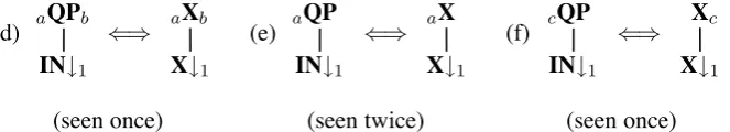
Option (a) may be sufficient for frequent rules, and will accurately model dependencies between different kinds of adjoining. However, it does not allow us to generalize to unseen patterns of adjoin-ing. Consider the low frequency situation depicted in Figure 6, rules (d)-(f). We may have seen this rule four times, once with adjoining site a, twice with adjoining sitesaandb, and once with a third adjoining sitec. The joint model will give a zero probability to unseen patterns of adjoining, e.g. no adjoining at any site or adjoining at site balone. Even if we use a discounting method to give a non-zero probability to unseen cases, we still have no way to distinguish one from another.

Option (b) allows us to learn reasonable esti-mates for these missing cases by separating out adjoining decisions and letting each speak for it-self. To properly learn non-zero probabilities for unseen cases5we use addksmoothing (k=1₂).

5_{For example, low frequency rules may have always been}

observed with a single adjoining pattern, and never without adjoining.

A weakness of this approach still remains: ad-joining is not a truly independent process, as we observe empirically in the data. In real data, fre-quent rules have many different observed adjoin-ing sites (10 or 20 in some cases), many of which represent already infrequent sites in combinations never seen together. To reduce the number of in-valid combinations produced, we only allow ad-joinings to be used at the same time if they have occurred together in the training data. This restric-tion makes it possible to do less adjoining than ob-served, but not more. For the example in Figure 6, in addition to the observed patterns, we would also allow sitebto be used alone, and we would allow no adjoinings, but we would not allow combina-tions of site c with either a or b. Later, we will see that this makes the decoding process more

ef-ficient.

Because both option (a) and (b) above have strengths and weaknesses, we also explore a third option which builds upon the strengths of each:

(c) A log-linear combination of the joint model and independent model. We assume the prob-ability has both a dependent and indepen-dent element, and learn the relative weight between them automatically

To help smooth this model we add two addi-tional binary features: one indicating adjoining patterns seen in data and one indicating previously unseen patterns.

4 Decoding

To translate with these rules, we do a monolingual parse using the foreign side of the rules (constrain-ing the search us(constrain-ing non-terminal labels from both sides), while keeping track of the English side string and structure for language modeling pur-poses. This produces all valid derivations of rules whose foreign side yield is the input string, from which we simply choose the one with the high-est log-linear model score. Though this process could be done directly using a specialized parsing algorithm, we note that these rules have weakly equivalent counterparts in the Synchronous Tree Substitution Grammar (STSG) and Tree-to-string transducer (xLNTs6_{) worlds, such that each STIG} rule can be translated into one equivalent rule, plus some helper rules to model the adjoin/no-adjoin

6_{xLNTs is shorthand for extended linear non-deleting}

Case 1: Case 2:

NP

NN

health

AlSHp

→

NN_↓1

⇐⇒ X

X_↓1

NP

JJ

national

NP

NN

defense

AldfAE AlwTnY

→

NP

JJ↓₁NP*

⇐⇒

X

X* X

X_↓1

(c) aNP

NN↓₁

⇐⇒ Xa

X↓₁

Figure 5: Selected rules learned in two cases. Rule (a) and (c) are considered the same rule, where (c) has the optional synchronous adjoining site marked with a. From these (limited) examples alone we would infer that adjective adjoining happens half the time, and is positioned before the noun in English, but after the noun in Arabic (thus the positioning of sitea).

(d) aQPb

IN↓₁

⇐⇒ aXb

X↓₁

(e) aQP

IN↓₁

⇐⇒ aX

X↓₁

(f) cQP

IN↓₁

⇐⇒ Xc

X↓₁

(seen once) (seen twice) (seen once)

Figure 6: For a low frequency rule, we may see only a few different adjoining patterns, but we want to infer more.

decision. Conversion to a better known and ex-plored formalism allows us to take advantage of existing code and algorithms. Here we describe the conversion process to xLNTs rules, though conversion to STSG is similar.

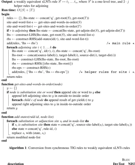
Algorithm 1 describes the process of converting one of our automatically learned STIG rules. On each side of the rule, we traverse the tree in a top-down, left-to-right order, recording words, substi-tution sites, and adjoining sites in the order en-countered (left adjoinings before the node’s chil-dren and right adjoinings after). We make these words and sites as the children under a single root node. The substitution sites are given states made up of a combination of their source and target la-bels as are the roots of non-adjoining rules. Ad-joining sites are labeled with a combination of the rule id and a site id. Adjoining rule roots are la-beled with a combination of the source and target root labels and the direction class. To allow for the adjoining/no-adjoining decision, two helper rules are created for each adjoining site, their root state a combination of the rule and site ids. One of these rules has only epsilon leaf nodes (representing no adjoining), while the other has leaf nodes and a state that match with the corresponding adjoining rule root (labeled with the site’s source and target labels and the direction class).

For each rule, the algorithm generates one main rule and pairs of helper rules to facilitate adjoining/non-adjoining. For computational effi -ciency reasons, our decoder supports neither silon rules nor non-binary rules. So we remove ep-silons using an exponential expansion of the rules: combine each main rule with an adjoining or non-adjoining helper rule for each adjunction site, then remove epsilon-only branches. Forkadjunction sites this could possibly results in2krules. But as discussed previously (at the end of Section 3.2), we only allow subsets of adjoining combinations seen in training data, so this number is substan-tially lower for large values ofk.

5 Experiments

Input: Synchronous TIG rulerwithjadjoining sites,S↔T, whereSandT are trees

Output: a weakly equivalent xLNTs ruleS! ↔t₁. . . t_n, whereS!is a one-level tree, and2·j helper rules for adjoining

Run time:O(|S|+|T|) begin

rules← {}, lhs-state←concat(‘q’, get-root(S), get-root(T)) site-and-word-list-s←get-sites-and-words-in-order(S) site-and-word-list-t←get-sites-and-words-in-order(T)

ifris adjoiningthenlhs-state←concat(lhs-state, get-adjoin-dir(S), get-adjoin-dir(T)) lhs←construct-LHS(lhs-state, get-root(S), site-and-word-list-s)

rhs←construct-RHS(add-states(id(r), site-and-word-list-t))

add(rules, ‘lhs↔rhs’) _{/* main rule */}

foreachadjoining sitei∈1. . . kdo

lhs-state←concat(‘q’, id(r),i), rhs-state←concat(‘q’, lhs-root)

lhs-root←concat(source-label(i), target-label(i), source-dir(i), target-dir(i)) lhs←construct-LHS(lhs-state, lhs-root, lhs-root)

rhs←construct-RHS({(rhs-state, lhs-root)}) rhs-eps←construct-RHS(!)

add(rules,{‘lhs↔rhs’, ‘lhs↔rhs-eps’}) _{/* helper rules for site} i _*/ return rules

end

functionget-sites-and-words-in-order(node)

y← {}

ifnode is substitution site or wordthenappend site or word toyelse

append left adjoining sites toyin outside-to-inside order

foreachchildcof nodedoappend result of get-yield(c) toy append right adjoining sites toyin inside-to-outside order returny

end

functionadd-states(ruld-id, node-list)

foreachsubstitution or adjunction sites_i and in node-listdo

ifs_iis substitution sitethenstate = concat(‘q’, source-site-label(s_i), target-site-label(s_i))

elsestate = concat(‘q’, rule-id,i) replaces_iwith (state,s_i)

return modified node-list

end

Algorithm 1: Conversion from synchronous TIG rules to weakly equivalent xLNTs rules

BLEU

description DevTest NIST06

(1) baseline: all required (GHKM minimal, head-out binarized parse trees) 48.0 47.0 (2) joint adjoining prob model alone (only observed adjoining patterns) 48.0 46.6 (3) independent adjoining prob model alone (only observed adjoining patterns) 48.1 46.7 (4) independent adjoining prob model alone (with new adjoining patterns) 48.5 47.6 (5) independent model alone + features (adjoining pattern, direction) 48.4 47.7 (6) log-linear combination of joint & independent models + features 48.7 47.8

made up of newswire documents drawn from the NIST MT evaluation data from 2004, 2005, and 2006 (GALE part). We use the newswire docu-ments from the NIST part of the 2006 evaluation data (765 sentences) as a held-out test set.

We train our feature weights using max-BLEU

(Och, 2003) and decode with a CKY-based de-coder that supports language model scoring di-rectly integrated into the search.

In addition to P_sub, P_adj, and Pif_adj, we use several other features in our log-linear model during decoding, including: lexical and phrase-based translation probabilities, a model similar to conditional probability on the trees (P(f_tree(rule)|e_tree(rule))), a probability model for generating the top tree non-terminal, a 5-gram language model7, and target length bonus. We also have several binary features—lexical rule, rule with missing or spurious content words—and several binary indicator features for specialized rules: unknown word rules; name, number, and date translation rules; and special fail-safe mono-tone translation rules in case of parse failures and extremely long sentences.

Table 1 shows the comparison between our baseline model (minimal GHKM on head-out bi-narized parse trees) and different models of ad-joining, measured with case-insensitive, NIST-tokenized BLEU(IBM definition). The top section

(lines 1–4) compares the joint adjoining ity model to the independent adjoining probabil-ity model and seen vs. unseen adjoining combi-nations. While the joint model results in a BLEU

score at the same level as our baseline (line 2), the independent model (line 4) improves BLEUby

+0.5 and +0.6, which are significant differences at the 95% confidence level. Since with the in-dependent model we introduce both new adjoin-ing patterns and a different probability model for adjoining (each site is independent), we also use the independent model with only previously seen adjoining patterns (line 3). The insignificant dif-ference in BLEU between lines 2 and 3 leads us to think that the new adjoining patterns are where the improvement comes from, rather than the in-dependent probability model alone.

We also test several other features and combi-nations. First, we add binary features to indicate a new adjoining combination vs. one previously

7_{The 5-gram LM was trained on 2 billion words of}

auto-matically selected collections taken from the NIST 08 allow-able data.

seen in data. We also add features to indicate the direction class of adjoining to test if there is a sys-tematic bias toward particular directions. These features cause no significant difference in score (line 5). We also add the joint-adjoining proba-bility as a feature, allowing it to be combined in a log-linear fashion with the independent probabil-ity (line 6). This results in our best BLEU gain: +0.7 and +0.8 over our non-adjoining baseline.

6 Conclusion

We have presented a novel method for learning the rules and probabilities for a new statistical, linguistically-informed, syntax-based MT model that allows for adjoining. We have described a method to translate using this model. And we have demonstrated that linguistically-motivated adjoin-ing improves the end-to-end MT results.

There are many potential directions for research to proceed. One possibility is to investigate other methods of making the required vs. optional de-cision, either using linguistic resources such as COMLEX or automatically learning the distinc-tion using EM (as done for tree binarizadistinc-tion by Wang et al. (2007)). In addition, most ideas pre-sented here are extendable to rules with linguistic trees on both sides (using insights from Lavie et al. (2008)). Also worth investigating is the direct integration of bilingual dictionaries into the gram-mar (as suggested by Shieber (2007)). Lastly, rule composition and different amounts of lexicaliza-tion (Galley et al., 2006; Marcu et al., 2006; De-Neefe et al., 2007) or context modeling (Mari˜no et al., 2006) have been successful with other mod-els.

Acknowledgments

We thank David Chiang for suggestions about adjoining models, Michael Pust and Jens-S¨onke V¨ockler for developing parts of the experimen-tal framework, and other colleagues at ISI for their helpful input. We also thank the anony-mous reviewers for insightful comments and sug-gestions. This research is financially supported under DARPA Contract No. HR0011-06-C-0022, BBN subcontract 9500008412.

References

David Chiang. 2003. Statistical parsing with an auto-matically extracted tree adjoining grammar. Data-Oriented Parsing.

Michael Collins. 2003. Head-driven statistical models for natural language parsing. Computational Lin-guistics, 29(4).

Steve DeNeefe, Kevin Knight, Wei Wang, and Daniel Marcu. 2007. What can syntax-based MT learn from phrase-based MT? InProc. EMNLP-CoNLL.

Alexander Fraser and Daniel Marcu. 2007. Getting the structure right for word alignment: LEAF. InProc. EMNLP-CoNLL.

Michel Galley, Mark Hopkins, Kevin Knight, and Daniel Marcu. 2004. What’s in a translation rule? InProc. HLT-NAACL.

Michel Galley, Jonathan Graehl, Kevin Knight, Daniel Marcu, Steve DeNeefe, Wei Wang, and Ignacio Thayer. 2006. Scalable inference and training of context-rich syntactic translation models. InProc. ACL.

Aravind K. Joshi, L. S. Levy, and M. Takahashi. 1975. Tree adjunct grammars. Journal of Computer and System Sciences, 10(1).

Aravind K. Joshi. 1985. How much context-sensitivity is necessary for characterizing structural descriptions—tree adjoining grammars. Natural Language Processing—Theoretical, Computational, and Psychological Perspectives.

Alon Lavie, Alok Parlikar, and Vamshi Ambati. 2008. Syntax-driven learning of sub-sentential translation equivalents and translation rules from parsed parallel corpora. InProc. SSST.

Daniel Marcu, Wei Wang, Abdessamad Echihabi, and Kevin Knight. 2006. SPMT: Statistical machine translation with syntactified target language phrases. InProc. EMNLP.

Mitchell P. Marcus, Beatrice Santorini, and Mary Ann Marcinkiewicz. 1993. Building a large annotated corpus of English: The Penn treebank. Computa-tional Linguistics, 19(2).

Jos´e B. Mari˜no, Rafael E. Banchs, Josep M. Crego, Adri`a de Gispert, Patrik Lambert, Jos´e A. R. Fonol-losa, and Marta R. Costa-juss`a. 2006. N-gram-based machine translation. Computational Linguis-tics, 32(4).

Rebecca Nesson, Stuart M. Shieber, and Alexander Rush. 2006. Induction of probabilistic synchronous tree-insertion grammars for machine translation. In

Proc. AMTA.

Franz Josef Och. 2003. Minimum error rate training in statistical machine translation. InProc. ACL.

Yves Schabes and Richard C. Waters. 1995. Tree insertion grammar: A cubic-time, parsable formal-ism that lexicalizes context-free grammar without changing the trees produced. Computational Lin-guistics, 21(4).

Stuart M. Shieber and Yves Schabes. 1990. Syn-chronous tree-adjoining grammars. InProc. COL-ING.

Stuart M. Shieber. 2007. Probabilistic synchronous tree-adjoining grammars for machine translation: The argument from bilingual dictionaries. InProc. SSST Wkshp., NAACL-HLT.

Kumar Vijay-Shanker. 1987.A study of tree adjoining grammars. Ph.D. thesis.