Domain Adaptation with Structural Correspondence Learning
John Blitzer Ryan McDonald Fernando Pereira
{blitzer|ryantm|pereira}@cis.upenn.edu
Department of Computer and Information Science, University of Pennsylvania 3330 Walnut Street, Philadelphia, PA 19104, USA
Abstract
Discriminative learning methods are widely used in natural language process-ing. These methods work best when their training and test data are drawn from the same distribution. For many NLP tasks, however, we are confronted with new domains in which labeled data is scarce or non-existent. In such cases, we seek to adapt existing models from a resource-rich source domain to a resource-poor target domain. We introduce structural
correspondence learning to automatically
induce correspondences among features from different domains. We test our tech-nique on part of speech tagging and show performance gains for varying amounts of source and target training data, as well as improvements in target domain parsing accuracy using our improved tagger.
1 Introduction
Discriminative learning methods are ubiquitous in natural language processing. Discriminative tag-gers and chunkers have been the state-of-the-art for more than a decade (Ratnaparkhi, 1996; Sha and Pereira, 2003). Furthermore, end-to-end sys-tems like speech recognizers (Roark et al., 2004) and automatic translators (Och, 2003) use increas-ingly sophisticated discriminative models, which generalize well to new data that is drawn from the same distribution as the training data.
However, in many situations we may have a
source domain with plentiful labeled training data,
but we need to process material from a target do-main with a different distribution from the source domain and no labeled data. In such cases, we must take steps to adapt a model trained on the source domain for use in the target domain (Roark and Bacchiani, 2003; Florian et al., 2004; Chelba
and Acero, 2004; Ando, 2004; Lease and Char-niak, 2005; Daum´e III and Marcu, 2006). This work focuses on using unlabeled data from both the source and target domains to learn a common feature representation that is meaningful across both domains. We hypothesize that a discrimi-native model trained in the source domain using this common feature representation will general-ize better to the target domain.
This representation is learned using a method we call structural correspondence learning (SCL). The key idea of SCL is to identify correspon-dences among features from different domains by modeling their correlations with pivot features. Pivot features are features which behave in the same way for discriminative learning in both do-mains. Non-pivot features from different domains which are correlated with many of the same pivot features are assumed to correspond, and we treat them similarly in a discriminative learner.
Even on the unlabeled data, the co-occurrence statistics of pivot and non-pivot features are likely to be sparse, and we must model them in a com-pact way. There are many choices for modeling co-occurrence data (Brown et al., 1992; Pereira et al., 1993; Blei et al., 2003). In this work we choose to use the technique of structural learn-ing (Ando and Zhang, 2005a; Ando and Zhang, 2005b). Structural learning models the correla-tions which are most useful for semi-supervised learning. We demonstrate how to adapt it for trans-fer learning, and consequently the structural part of structural correspondence learning is borrowed from it.1
SCL is a general technique, which one can ap-ply to feature based classifiers for any task. Here,
1Structural learning is different from learning with struc-tured outputs, a common paradigm for discriminative nat-ural language processing models. To avoid terminologi-cal confusion, we refer throughout the paper to a specific structural learning method, alternating structural optimiza-tion (ASO) (Ando and Zhang, 2005a).
(a) Wall Street Journal
DT JJ VBZ DT NN IN DT JJ NN
The clash is a sign of a new toughness
CC NN IN NNP POS JJ JJ NN .
and divisiveness in Japan ’s once-cozy financial circles . (b) MEDLINE
DT JJ VBN NNS IN DT NN NNS VBP
The oncogenic mutated forms of the ras proteins are
RB JJ CC VBP IN JJ NN NN .
[image:2.595.118.498.74.178.2]constitutively active and interfere with normal signal transduction . Figure 1: Part of speech-tagged sentences from both corpora
we investigate its use in part of speech (PoS) tag-ging (Ratnaparkhi, 1996; Toutanova et al., 2003). While PoS tagging has been heavily studied, many domains lack appropriate training corpora for PoS tagging. Nevertheless, PoS tagging is an impor-tant stage in pipelined language processing sys-tems, from information extractors to speech syn-thesizers. We show how to use SCL to transfer a PoS tagger from the Wall Street Journal (financial news) to MEDLINE (biomedical abstracts), which use very different vocabularies, and we demon-strate not only improved PoS accuracy but also improved end-to-end parsing accuracy while using the improved tagger.
An important but rarely-explored setting in do-main adaptation is when we have no labeled training data for the target domain. We first demonstrate that in this situation SCL significantly improves performance over both supervised and semi-supervised taggers. In the case when some in-domain labeled training data is available, we show how to use SCL together with the classifier combination techniques of Florian et al. (2004) to achieve even greater performance.
In the next section, we describe a motivating example involving financial news and biomedical data. Section 3 describes the structural correspon-dence learning algorithm. Sections 6 and 7 report results on adapting from the Wall Street Journal to MEDLINE. We discuss related work on domain adaptation in section 8 and conclude in section 9.
2 A Motivating Example
Figure 1 shows two PoS-tagged sentences, one each from the Wall Street Journal (hereafter WSJ) and MEDLINE. We chose these sentences for two reasons. First, we wish to visually emphasize the difference between the two domains. The vocab-ularies differ significantly, and PoS taggers suf-fer accordingly. Second, we want to focus on the
(a) An ambiguous instance JJ vs. NN
with normal signal transduction
(b) MEDLINE occurrences of signal, together with pivot features
the signal required to stimulatory signal from essential signal for
(c) Corresponding WSJ words, together with pivot features
[image:2.595.315.529.219.331.2]of investment required of buyouts from buyers to jail for violating Figure 2: Correcting an incorrect biomedical tag. Corresponding words are in bold, and pivot fea-tures are italicized
phrase “with normal signal transduction” from the MEDLINE sentence, depicted in Figure 2(a). The word “signal” in this sentence is a noun, but a tag-ger trained on the WSJ incorrectly classifies it as an adjective. We introduce the notion of pivot fea-tures. Pivot features are features which occur fre-quently in the two domains and behave similarly in both. Figure 2(b) shows some pivot features that occur together with the word “signal” in our biomedical unlabeled data. In this case our pivot features are all of type <the token on the right>. Note that “signal” is unambiguously a noun in these contexts. Adjectives rarely precede past tense verbs such as “required” or prepositions such as “from” and “for”.
We now search for occurrences of the pivot fea-tures in the WSJ. Figure 2(c) shows some words that occur together with the pivot features in the WSJ unlabeled data. Note that “investment”, “buy-outs”, and “jail” are all common nouns in the financial domain. Furthermore, since we have la-beled WSJ data, we expect to be able to label at least some of these nouns correctly.
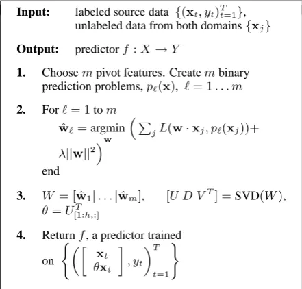
Input: labeled source data {(xt, yt)Tt=1}, unlabeled data from both domains{xj} Output: predictorf:X→Y
1. Choosempivot features. Creatembinary prediction problems,p`(x), `= 1. . . m 2. For`= 1tom
ˆ
w`=argmin
w “
P
jL(w·xj, p`(xj))+
λ||w||2
”
end
3. W = [ ˆw1|. . .|wˆm], [U D VT] =SVD(W),
θ=UT
[1:h,:]
4. Returnf, a predictor trained on
( „»
xt
θxi
– , yt
«T
t=1
[image:3.595.72.293.68.279.2])
Figure 3: SCL Algorithm
we want the pivot features to model the fact that in the biomedical domain, the word signal behaves similarly to the words investments, buyouts and
jail in the financial news domain. In practice, we
use this technique to find correspondences among all features, not just word features.
3 Structural Correspondence Learning
Structural correspondence learning involves a source domain and a target domain. Both domains have ample unlabeled data, but only the source do-main has labeled training data. We refer to the task for which we have labeled training data as the
su-pervised task. In our experiments, the susu-pervised
task is part of speech tagging. We require that the inputxin both domains be a vector of binary fea-tures from a finite feature space. The first step of SCL is to define a set of pivot features on the unla-beled data from both domains. We then use these pivot features to learn a mappingθfrom the orig-inal feature spaces of both domains to a shared, low-dimensional real-valued feature space. A high inner product in this new space indicates a high de-gree of correspondence.
During supervised task training, we use both the transformed and original features from the source domain. During supervised task testing, we use the both the transformed and original features from the target domain. If we learned a good map-ping θ, then the classifier we learn on the source domain will also be effective on the target domain. The SCL algorithm is given in Figure 3, and the remainder of this section describes it in detail.
3.1 Pivot Features
Pivot features should occur frequently in the un-labeled data of both domains, since we must esti-mate their covariance with non-pivot features ac-curately, but they must also be diverse enough to adequately characterize the nuances of the su-pervised task. A good example of this tradeoff are determiners in PoS tagging. Determiners are good pivot features, since they occur frequently in any domain of written English, but choosing
only determiners will not help us to discriminate
between nouns and adjectives. Pivot features cor-respond to the auxiliary problems of Ando and Zhang (2005a).
In section 2, we showed example pivot fea-tures of type <the token on the right>. We also use pivot features of type<the token on the left> and <the token in the middle>. In practice there are many thousands of pivot features, corresponding to instantiations of these three types for frequent words in both do-mains. We choosempivot features, which we in-dex with`.
3.2 Pivot Predictors
From each pivot feature we create a binary clas-sification problem of the form “Does pivot fea-ture ` occur in this instance?”. One such ex-ample is “Is <the token on the right>
required?” These binary classification problems
can be trained from the unlabeled data, since they merely represent properties of the input. If we rep-resent our features as a binary vector x, we can solve these problems usingmlinear predictors.
f`(x) =sgn( ˆw`·x), `= 1. . . m
Note that these predictors operate on the original feature space. This step is shown in line 2 of Fig-ure 3. Here L(p, y) is a real-valued loss func-tion for binary classificafunc-tion. We follow Ando and Zhang (2005a) and use the modified Huber loss.
Since each instance contains features which are totally predictive of the pivot feature (the feature itself), we never use these features when making the binary prediction. That is, we do not use any feature derived from the right word when solving a right token pivot predictor.
pivot predictor is positive, then feature z is posi-tively correlated with pivot feature `. Since pivot features occur frequently in both domains, we ex-pect non-pivot features from both domains to be correlated with them. If two non-pivot features are correlated in the same way with many of the same pivot features, then they have a high degree of cor-respondence. Finally, observe that wˆ` is a linear projection of the original feature space ontoR.
3.3 Singular Value Decomposition
Since each pivot predictor is a projection ontoR, we could create m new real-valued features, one for each pivot. For both computational and statis-tical reasons, though, we follow Ando and Zhang (2005a) and compute a low-dimensional linear ap-proximation to the pivot predictor space. Let W
be the matrix whose columns are the pivot pre-dictor weight vectors. Now let W = U DVT be the singular value decomposition of W, so that
θ = U[1:Th,:] is the matrix whose rows are the top left singular vectors ofW.
The rows ofθare the principal pivot predictors, which capture the variance of the pivot predictor space as best as possible inhdimensions. Further-more, θ is a projection from the original feature space ontoRh. That is,θxis the desired mapping to the (low dimensional) shared feature represen-tation. This is step 3 of Figure 3.
3.4 Supervised Training and Inference
To perform inference and learning for the super-vised task, we simply augment the original fea-ture vector with feafea-tures obtained by applying the mapping θ. We then use a standard discrimina-tive learner on the augmented feature vector. For training instance t, the augmented feature vector will contain all the original features xt plus the new shared featuresθxt. If we have designed the pivots well, thenθshould encode correspondences among features from different domains which are important for the supervised task, and the classi-fier we train using these new features on the source domain will perform well on the target domain.
4 Model Choices
Structural correspondence learning uses the tech-niques of alternating structural optimization (ASO) to learn the correlations among pivot and non-pivot features. Ando and Zhang (2005a) de-scribe several free paramters and extensions to
ASO, and we briefly address our choices for these here. We seth, the dimensionality of our low-rank representation to be 25. As in Ando and Zhang (2005a), we observed that setting h between 20 and 100 did not change results significantly, and a lower dimensionality translated to faster run-time. We also implemented both of the extensions de-scribed in Ando and Zhang (2005a). The first is to only use positive entries in the pivot predictor weight vectors to compute the SVD. This yields a sparse representation which saves both time and space, and it also performs better. The second is to compute block SVDs of the matrixW, where one block corresponds to one feature type. We used the same 58 feature types as Ratnaparkhi (1996). This gave us a total of1450projection features for both semisupervised ASO and SCL.
We found it necessary to make a change to the ASO algorithm as described in Ando and Zhang (2005a). We rescale the projection features to al-low them to receive more weight from a regular-ized discriminative learner. Without any rescaling, we were not able to reproduce the original ASO results. The rescaling parameter is a single num-ber, and we choose it using heldout data from our source domain. In all our experiments, we rescale our projection features to have averageL1norm on the training set five times that of the binary-valued features.
Finally, we also make one more change to make optimization faster. We select only half of the ASO features for use in the final model. This is done by running a few iterations of stochas-tic gradient descent on the PoS tagging problem, then choosing the features with the largest weight-variance across the different labels. This cut in half training time and marginally improved perfor-mance in all our experiments.
5 Data Sets and Supervised Tagger
5.1 Source Domain: WSJ
We used sections 02-21 of the Penn Treebank (Marcus et al., 1993) for training. This resulted in 39,832 training sentences. For the unlabeled data, we used 100,000 sentences from a 1988 subset of the WSJ.
5.2 Target Domain: Biomedical Text
varia-company
transaction
investors
officials pretty your
short-term political
receptors mutation
assays
lesions functional
transient neuronal
metastatic
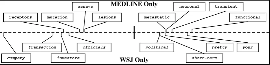
[image:5.595.74.523.67.176.2]WSJ Only MEDLINE Only
Figure 4: An example projection of word features ontoR. Words on the left (negative valued) behave similarly to each other for classification, but differently from words on the right (positive valued). The projection distinguishes nouns from adjectives and determiners in both domains.
tions and mutations. For labeled training and test-ing purposes we use 1061 sentences that have been annotated by humans as part of the Penn BioIE project (PennBioIE, 2005). We use the same 561-sentence test set in all our experiments. The part-of-speech tag set for this data is a superset of the Penn Treebank’s including the two new tags HYPH (for hyphens) and AFX (for common post-modifiers of biomedical entities such as genes). These tags were introduced due to the importance of hyphenated entities in biomedical text, and are used for 1.8% of the words in the test set. Any tagger trained only on WSJ text will automatically predict wrong tags for those words.
5.3 Supervised Tagger
Since SCL is really a method for inducing a set of cross-domain features, we are free to choose any feature-based classifier to use them. For our experiments we use a version of the discrim-inative online large-margin learning algorithm MIRA (Crammer et al., 2006). MIRA learns and outputs a linear classification score,s(x,y;w) =
w·f(x,y), where the feature representationfcan contain arbitrary features of the input, including the correspondence features described earlier. In particular, MIRA aims to learn weights so that the score of correct output, yt, for input xt is separated from the highest scoring incorrect out-puts2, with a margin proportional to their Ham-ming losses. MIRA has been used successfully for both sequence analysis (McDonald et al., 2005a) and dependency parsing (McDonald et al., 2005b). As with any structured predictor, we need to factor the output space to make inference tractable. We use a first-order Markov factorization, allow-ing for an efficient Viterbi inference procedure.
2
We fix the number of high scoring incorrect outputs to 5.
6 Visualizingθ
In section 2 we claimed that good representations should encode correspondences between words like “signal” from MEDLINE and “investment” from the WSJ. Recall that the rows of θare pro-jections from the original feature space onto the real line. Here we examine word features under these projections. Figure 4 shows a row from the matrixθ. Applying this projection to a word gives a real value on the horizontal dashed line axis. The words below the horizontal axis occur only in the WSJ. The words above the axis occur only in MEDLINE. The verticle line in the mid-dle represents the value zero. Ticks to the left or right indicate relative positive or negative values for a word under this projection. This projection discriminates between nouns (negative) and adjec-tives (positive). A tagger which gives high pos-itive weight to the features induced by applying this projection will be able to discriminate among the associated classes of biomedical words, even when it has never observed the words explicitly in the WSJ source training set.
7 Empirical Results
(a)
100 500 1k 5k 40k 75
80 85 90
Results for 561 MEDLINE Test Sentences
Number of WSJ Training Sentences
Accuracy
supervised semi−ASO SCL
(b) Accuracy on 561-sentence test set Words Model All Unknown Ratnaparkhi (1996) 87.2 65.2
supervised 87.9 68.4 semi-ASO 88.4 70.9 SCL 88.9 72.0
(c) Statistical Significance (McNemar’s)
for all words
Null Hypothesis p-value
[image:6.595.85.497.72.268.2]semi-ASO vs. super 0.0015 SCL vs. super 2.1×10⁻¹² SCL vs. semi-ASO 0.0003
Figure 5: PoS tagging results with no target labeled training data
(a)
50 100 200 500
86 88 90 92 94 96
Number of MEDLINE Training Sentences
Accuracy
Results for 561 MEDLINE Test Sentences
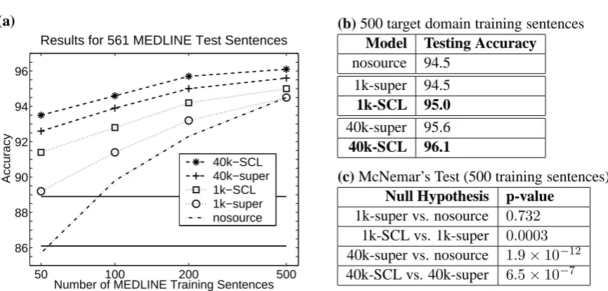
40k−SCL 40k−super 1k−SCL 1k−super nosource
(b) 500 target domain training sentences Model Testing Accuracy
nosource 94.5 1k-super 94.5
1k-SCL 95.0
40k-super 95.6
40k-SCL 96.1
(c) McNemar’s Test (500 training sentences) Null Hypothesis p-value
[image:6.595.77.512.76.462.2]1k-super vs. nosource 0.732 1k-SCL vs. 1k-super 0.0003 40k-super vs. nosource 1.9×10⁻¹² 40k-SCL vs. 40k-super 6.5×10⁻⁷
Figure 6: PoS tagging results with no target labeled training data
tagger improves the performance of a dependency parser on the target domain.
7.1 No Target Labeled Training Data
For the results in this section, we trained a structural correspondence learner with 100,000 sentences of unlabeled data from the WSJ and 100,000 sentences of unlabeled biomedical data. We use as pivot features words that occur more than 50 times in both domains. The supervised baseline does not use unlabeled data. The ASO baseline is an implementation of Ando and Zhang (2005b). It uses 200,000 sentences of unlabeled MEDLINE data but no unlabeled WSJ data. For ASO we used as auxiliary problems words that oc-cur more than 500 times in the MEDLINE unla-beled data.
Figure 5(a) plots the accuracies of the three models with varying amounts of WSJ training data. With one hundred sentences of training data, structural correspondence learning gives a 19.1% relative reduction in error over the super-vised baseline, and it consistently outperforms both baseline models. Figure 5(b) gives results for 40,000 sentences, and Figure 5(c) shows cor-responding significance tests, with p < 0.05 be-ing significant. We use a McNemar paired test for labeling disagreements (Gillick and Cox, 1989). Even when we use all the WSJ training data avail-able, the SCL model significantly improves accu-racy over both the supervised and ASO baselines.
[image:6.595.80.513.294.501.2]Of thirteen thousand test instances, approximately three thousand were unknown. For unknown words, SCL gives a relative reduction in error of 19.5% over Ratnaparkhi (1996), even with 40,000 sentences of source domain training data.
7.2 Some Target Labeled Training Data
In this section we give results for small amounts of target domain training data. In this case, we make use of the out-of-domain data by using features of the source domain tagger’s predictions in training and testing the target domain tagger (Florian et al., 2004). Though other methods for incorporating small amounts of training data in the target domain were available, such as those proposed by Chelba and Acero (2004) and by Daum´e III and Marcu (2006), we chose this method for its simplicity and consistently good performance. We use as features the current predicted tag and all tag bigrams in a 5-token window around the current token.
Figure 6(a) plots tagging accuracy for varying amounts of MEDLINE training data. The two horizontal lines are the fixed accuracies of the SCL WSJ-trained taggers using one thousand and forty thousand sentences of training data. The five learning curves are for taggers trained with vary-ing amounts of target domain trainvary-ing data. They use features on the outputs of taggers from sec-tion 7.1. The legend indicates the kinds of features used in the target domain (in addition to the stan-dard features). For example, “40k-SCL” means that the tagger uses features on the outputs of an SCL source tagger trained on forty thousand sen-tences of WSJ data. “nosource” indicates a tar-get tagger that did not use any tagger trained on the source domain. With 1000 source domain sen-tences and 50 target domain sensen-tences, using SCL tagger features gives a 20.4% relative reduction in error over using supervised tagger features and a 39.9% relative reduction in error over using no source features.
Figure 6(b) is a table of accuracies for 500 tar-get domain training sentences, and Figure 6(c) gives corresponding significance scores. With 1000 source domain sentences and 500 target do-main sentences, using supervised tagger features gives no improvement over using no source fea-tures. Using SCL features still does, however.
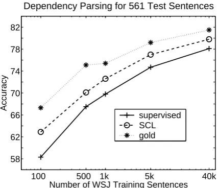
7.3 Improving Parser Performance
We emphasize the importance of PoS tagging in a pipelined NLP system by incorporating our SCL
100 500 1k 5k 40k 58
62 66 70 74 78 82
Dependency Parsing for 561 Test Sentences
Number of WSJ Training Sentences
Accuracy
[image:7.595.310.524.67.251.2]supervised SCL gold
Figure 7: Dependency parsing results using differ-ent part of speech taggers
tagger into a WSJ-trained dependency parser and and evaluate it on MEDLINE data. We use the parser described by McDonald et al. (2005b). That parser assumes that a sentence has been PoS-tagged before parsing. We train the parser and PoS tagger on the same size of WSJ data.
Figure 7 shows dependency parsing accuracy on our 561-sentence MEDLINE test set. We parsed the sentences using the PoS tags output by our source domain supervised tagger, the SCL tagger from subsection 7.1, and the gold PoS tags. All of the differences in this figure are significant ac-cording to McNemar’s test. The SCL tags consis-tently improve parsing performance over the tags output by the supervised tagger. This is a rather in-direct method of improving parsing performance with SCL. In the future, we plan on directly incor-porating SCL features into a discriminative parser to improve its adaptation properties.
8 Related Work
maximum entropy target domain classifier. The prior is Gaussian with mean equal to the weights of the source domain classifier. Daum´e III and Marcu (2006) use an empirical Bayes model to es-timate a latent variable model grouping instances into domain-specific or common across both do-mains. They also jointly estimate the parameters of the common classification model and the do-main specific classification models. Our work fo-cuses on finding a common representation for
fea-tures from different domains, not instances. We
believe this is an important distinction, since the same instance can contain some features which are common across domains and some which are do-main specific.
The key difference between the previous four pieces of work and our own is the use of unlabeled data. We do not require labeled training data in the new domain to demonstrate an improvement over our baseline models. We believe this is essen-tial, since many domains of application in natural language processing have no labeled training data. Lease and Charniak (2005) adapt a WSJ parser to biomedical text without any biomedical tree-banked data. However, they assume other labeled resources in the target domain. In Section 7.3 we give similar parsing results, but we adapt a source domain tagger to obtain the PoS resources.
To the best of our knowledge, SCL is the first method to use unlabeled data from both domains for domain adaptation. By using just the unlabeled data from the target domain, however, we can view domain adaptation as a standard semisupervised learning problem. There are many possible ap-proaches for semisupservised learning in natural language processing, and it is beyond the scope of this paper to address them all. We chose to compare with ASO because it consistently outper-forms cotraining (Blum and Mitchell, 1998) and clustering methods (Miller et al., 2004). We did run experiments with the top-k version of ASO (Ando and Zhang, 2005a), which is inspired by cotraining but consistently outperforms it. This did not outperform the supervised method for do-main adaptation. We speculate that this is because biomedical and financial data are quite different. In such a situation, bootstrapping techniques are likely to introduce too much noise from the source domain to be useful.
Structural correspondence learning is most sim-ilar to that of Ando (2004), who analyzed a
situation with no target domain labeled data. Her model estimated co-occurrence counts from source unlabeled data and then used the SVD of this matrix to generate features for a named en-tity recognizer. Our ASO baseline uses unlabeled data from the target domain. Since this consis-tently outperforms unlabeled data from only the
source domain, we report only these baseline
re-sults. To the best of our knowledge, this is the first work to use unlabeled data from both domains to find feature correspondences.
One important advantage that this work shares with Ando (2004) is that an SCL model can be easily combined with all other domain adaptation techniques (Section 7.2). We are simply induc-ing a feature representation that generalizes well across domains. This feature representation can then be used in all the techniques described above.
9 Conclusion
Structural correspondence learning is a marriage of ideas from single domain semi-supervised learning and domain adaptation. It uses unla-beled data and frequently-occurring pivot features from both source and target domains to find corre-spondences among features from these domains. Finding correspondences involves estimating the correlations between pivot and non-pivot feautres, and we adapt structural learning (ASO) (Ando and Zhang, 2005a; Ando and Zhang, 2005b) for this task. SCL is a general technique that can be ap-plied to any feature-based discriminative learner.
We showed results using SCL to transfer a PoS tagger from the Wall Street Journal to a corpus of MEDLINE abstracts. SCL consistently out-performed both supervised and semi-supervised learning with no labeled target domain training data. We also showed how to combine an SCL tagger with target domain labeled data using the classifier combination techniques from Florian et al. (2004). Finally, we improved parsing perfor-mance in the target domain when using the SCL PoS tagger.
learning when we have labeled data from both source and target domains. In particular, the la-beled data of both domains, not just the unlala-beled data, should influence the learned representations.
Acknowledgments
We thank Rie Kubota Ando and Tong Zhang for their helpful advice on ASO, Steve Carroll and Pete White of The Children’s Hospital of Philadelphia for providing the MEDLINE data, and the PennBioIE annotation team for the anno-tated MEDLINE data used in our test sets. This material is based upon work partially supported by the Defense Advanced Research Projects Agency (DARPA) under Contract No. NBCHD030010. Any opinions, findings, and conclusions or rec-ommendations expressed in this material are those of the author(s) and do not necessarily reflect the views of the DARPA or the Department of Interior-National Business Center (DOI-NBC). Additional support was provided by NSF under ITR grant EIA-0205448.
References
R. Ando and T. Zhang. 2005a. A framework for learn-ing predictive structures from multiple tasks and un-labeled data. JMLR, 6:1817–1853.
R. Ando and T. Zhang. 2005b. A high-performance semi-supervised learning method for text chunking. In ACL.
R. Ando. 2004. Exploiting unannotated corpora for tagging and chunking. In ACL. Short paper.
D. Blei, A. Ng, and M. Jordan. 2003. Latent dirichlet allocation. JMLR, 3:993–1022.
A. Blum and T. Mitchell. 1998. Combining labeled and unlabeled data with co-training. In Workshop
on Computational Learning Theory.
P. Brown, V. Della Pietra, P. deSouza, J. Lai, and R. Mercer. 1992. Class-based n-gram models of natural language. Computational Linguistics,
18(4):467–479.
C. Chelba and A. Acero. 2004. Adaptation of maxi-mum entropy capitalizer: Little data can help a lot. In EMNLP.
K. Crammer, Dekel O, J. Keshet, S. Shalev-Shwartz, and Y. Singer. 2006. Online passive-aggressive al-gorithms. JMLR, 7:551–585.
H. Daum´e III and D. Marcu. 2006. Domain adaptation for statistical classifiers. JAIR.
R. Florian, H. Hassan, A.Ittycheriah, H. Jing, N. Kambhatla, X. Luo, N. Nicolov, and S. Roukos. 2004. A statistical model for multilingual entity de-tection and tracking. In of HLT-NAACL.
L. Gillick and S. Cox. 1989. Some statistical issues in the comparison of speech recognition algorithms. In
ICASSP.
R. Kuhn, P. Nguyen, J.C. Junqua, L. Goldwasser, N. Niedzielski, S. Fincke, K. Field, and M. Con-tolini. 1998. Eigenvoices for speaker adaptation. In ICSLP.
M. Lease and E. Charniak. 2005. Parsing biomedical literature. In IJCNLP.
M. Marcus, B. Santorini, and M. Marcinkiewicz. 1993. Building a large annotated corpus of En-glish: The Penn Treebank. Computational
Linguis-tics, 19(2):313–330.
R. McDonald, K. Crammer, and F. Pereira. 2005a. Flexible text segmentation with structured multil-abel classification. In HLT-EMNLP.
R. McDonald, K. Crammer, and F. Pereira. 2005b. On-line large-margin training of dependency parsers. In
ACL.
S. Miller, J. Guinness, and A. Zamanian. 2004. Name tagging with word clusters and discriminative train-ing. In HLT-NAACL.
F. Och. 2003. Minimum error rate training in statistical machine translation. In Proc. of ACL.
PennBioIE. 2005. Mining The Bibliome Project. http://bioie.ldc.upenn.edu/.
F. Pereira, N. Tishby, and L. Lee. 1993. Distributional clustering of english words. In ACL.
A. Ratnaparkhi. 1996. A maximum entropy model for part-of-speech tagging. In EMNLP.
B. Roark and M. Bacchiani. 2003. Supervised and unsupervised PCFG adaptation to novel domains. In
HLT-NAACL.
B. Roark, M. Saraclar, M. Collins, and M. Johnson. 2004. Discriminative language modeling with con-ditional random fields and the perceptron algorithm. In ACL.
F. Sha and F. Pereira. 2003. Shallow parsing with con-ditional random fields. In HLT-NAACL.