Noise Contrastive Estimation and Negative Sampling for Conditional Models: Consistency and Statistical Efficiency

Noise Contrastive Estimation and Negative Sampling for Conditional

Models: Consistency and Statistical Efficiency

Zhuang Ma

University of Pennsylvania⇤ [email protected]

Michael Collins

Google AI Language and Columbia University†

[email protected]

Abstract

Noise Contrastive Estimation (NCE) is a pow-erful parameter estimation method for log-linear models, which avoids calculation of the partition function or its derivatives at each training step, a computationally demanding step in many cases. It is closely related to negative sampling methods, now widely used in NLP. This paper considers NCE-based es-timation ofconditional models. Conditional models are frequently encountered in practice; however there has not been a rigorous theo-retical analysis of NCE in this setting, and we will argue there are subtle but important ques-tions when generalizing NCE to the condi-tional case. In particular, we analyze two vari-ants of NCE for conditional models: one based on a classification objective, the other based on a ranking objective. We show that the ranking-based variant of NCE gives consistent param-eter estimates under weaker assumptions than the classification-based method; we analyze the statistical efficiency of the ranking-based and classification-based variants of NCE; fi-nally we describe experiments on synthetic data and language modeling showing the ef-fectiveness and trade-offs of both methods.

1 Introduction

This paper considers parameter estimation in con-ditional models of the form

p(y|x;✓) = exp (s(x, y;✓))

Z(x;✓) (1)

wheres(x, y;✓)is the unnormalized score of label

yin conjunction with inputxunder parameters✓,

Y is a finite set of possible labels, andZ(x;✓) = P

y2Yexp (s(x, y;✓))is the partition function for

inputxunder parameters✓.

It is hard to overstate the importance of models of this form in NLP. In log-linear models, includ-ing both the original work on maximum-entropy models (Berger et al., 1996), and later work on conditional random fields (Lafferty et al., 2001),

⇤_{Part of this work done at Google.}

†_{Work done at Google.}

the scoring functions(x, y;✓) =✓_·f(x, y)where f(x, y) 2 Rd _{is a feature vector, and✓ 2 R}d_are the parameters of the model. In more recent work on neural networks the functions(x, y;✓)is a non-linear function. In Word2Vec the scoring function is s(x, y;✓) = ✓x·✓0y where y is a word in the context of wordx, and✓x 2 Rdand✓y0 2Rdare “inside” and “outside” word embeddingsxandy. In many NLP applications the set Y is large. Maximum likelihood estimation (MLE) of the pa-rameters ✓ requires calculation of Z(x;✓) or its derivatives at each training step, thereby requiring a summation over all members ofY, which can be computationally expensive. This has led to many authors considering alternative methods, often re-ferred to as “negative sampling methods”, where a modified training objective is used that does not require summation overY on each example. In-stead negative examples are drawn from some dis-tribution, and a objective function is derived based on binary classification or ranking. Prominent ex-amples are the binary objective used in word2vec ((Mikolov et al.,2013), see also (Levy and Gold-berg, 2014)), and the Noise Contrastive Estima-tion methods of (Mnih and Teh,2012;Jozefowicz et al.,2016) for estimation of language models.

In spite of the centrality of negative sampling methods, they are arguably not well understood from a theoretical standpoint. There are clear connections to noise contrastive estimation (NCE) (Gutmann and Hyv¨arinen,2012), a negative sam-pling method for parameter estimation in joint

models of the form

p(y) = exp (s(y;✓))

Z(✓) ; Z(✓) = X

y2Y

exp (s(y;✓))

(2) However there has not been a rigorous theoretical analysis of NCE in the estimation of conditional

param-eter of the model (Gutmann and Hyv¨arinen,2012) whereas the conditional model in Eq1has a sepa-rate partition functionZ(x;✓)for each value ofx. This difference is critical.

We show the following (throughout we define K 1 to be the number of negative examples

sampled per training example):

•For anyK 1, a binary classification variant

of NCE, as used by (Mnih and Teh,2012;Mikolov et al.,2013), gives consistent parameter estimates under the assumption thatZ(x;✓)is constant with

respect tox(i.e.,Z(x;✓) =H(✓)for some

func-tion H). Equivalently, the method is consistent under the assumption that the function s(x, y;✓)

is powerful enough to incorporatelogZ(x;✓).

• For anyK 1, a ranking-based variant of

NCE, as used by (Jozefowicz et al.,2016), gives consistent parameter estimates under the much weaker assumption thatZ(x;✓)can vary with x. Equivalently, there is no need for s(x, y;✓) to be

powerful enough to incorporatelogZ(x;✓).

• We analyze the statistical efficiency of the ranking-based and classification-based NCE ants. Under respective assumptions, both vari-ants achieve Fisher efficiency (the same asymp-totic mean square error as the MLE) asK _{! 1}.

• We discuss application of our results to ap-proaches of (Mnih and Teh,2012;Mikolov et al.,

2013;Levy and Goldberg,2014;Jozefowicz et al.,

2016) giving a unified account of these methods. • We describe experiments on synthetic data and language modeling evaluating the effective-ness of the two NCE variants.

2 Basic Assumptions

We assume the following setup throughout: •We have setsX andY, whereX,Yare finite. • There is some unknown joint distribution pX,Y(x, y)wherex 2X andy 2 Y. We assume that the marginal distributions satisfypX(x) > 0 for allx_2X andpY(y)>0for ally2Y.

• We have training examples {x(i), y(i)}n i=1

drawn I.I.D. frompX,Y(x, y).

• We have a scoring function s(x, y;✓) where ✓ are the parameters of the model. For example,

s(x, y;✓)may be defined by a neural network.

•We use⇥to refer to the parameter space. We assume that⇥✓Rd_{for some integerd.}

• We use pN(y) to refer to a distribution from which negative examples are drawn in the NCE approach. We assume thatpN satisfiespN(y)>0 for ally_2Y.

We will consider estimation under the following two assumptions:

Assumption 2.1 There exists some parameter value ✓⇤ 2 ⇥such that for all(x, y) 2 X ⇥Y,

p_Y|X(y_|x) = exp(s(x, y;✓⇤))

Z(x;✓⇤₎ (3)

whereZ(x;✓⇤) =P_y2Yexp(s(x, y;✓⇤)).

Assumption 2.2 There exists some parameter value ✓⇤ 2 ⇥, and a constant ⇤ 2 R, such that for all(x, y)_{2X ⇥Y},

pY|X(y|x) = exp (s(x, y;✓⇤) ⇤). (4)

Assumption 2.2 is stronger than Assump-tion 2.1. It requires logZ(x;✓⇤) ⌘ ⇤ _{for all} x _2X, that is, the conditional distribution is per-fectly self-normalized. Under Assumption2.2, it must be the case that8x2X

X

y

p_Y|X(y_|x) =X

y

exp_{s(x, y;✓⇤) ⇤_}= 1

There are|X | constraints but onlyd+ 1 free

pa-rameters. Therefore self-normalization is a non-trivial assumption when|X | d. In the case of language modeling,|X | =_|V_|k _{d+ 1, where} |V|is the vocabulary size and k is the length of the context. The number of constraints grows ex-ponentially fast.

Given a scoring functions(x, y;✓)that satisfies

assumption2.1, we can derive a scoring function s0_{that satisfies assumption2.2by defining}

s0(x, y;✓,_{cx:x2X }) =s(x, y;✓) cx

wherecx 2 Ris a parameter for historyx. Thus we introduce a new parametercxfor each possible historyx. This is the most straightforward exten-sion of NCE to the conditional case; it is used by (Mnih and Teh, 2012). It has the clear drawback however of introducing a large number of addi-tional parameters to the model.

3 Two Estimation Algorithms

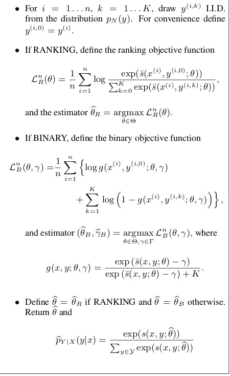
Figure 1 shows two NCE-based parameter esti-mation algorithms, based respectively on binary objective and ranking objective. The input to either algorithm is a set of training examples {x(i), y(i)}n

i=1, a parameterKspecifying the

a distribution pN(·) from which negative exam-ples are sampled. The algorithms differ only in the choice of objective function being optimized: Ln_B for binary objective, andLn

Rfor ranking objective. Binary objective essentially corresponds to a prob-lem where the scoring function s(x, y;✓) is used

to construct a binary classifier that discriminates between positive and negative examples. Rank-ing objective corresponds to a problem where the scoring functions(x, y;✓)is used to rank the true

labely(i)above negative examplesy(i,1). . . y(i,K) for the inputx(i).

Our main result is as follows:

Theorem 3.1 (Informal: see section 4for a for-mal statement.) For any K 1, the binary

classification-based algorithm in figure 1 is con-sistent under Assumption 2.2, but is not always consistent under the weaker Assumption2.1. For anyK 1, the ranking-based algorithm in

fig-ure1is consistent under either Assumption2.1or Assumption2.2. Both algorithms achieve the same statistical efficiency as the maximum-likelihood estimate asK _{! 1}.

The remainder of this section gives a sketch of the argument underlying consistency, and dis-cusses use of the two algorithms in previous work.

3.1 A Sketch of the Consistency Argument for the Ranking-Based Algorithm

In this section, in order to develop intuition under-lying the ranking algorithm, we give a proof sketch of the following theorem:

Theorem 3.2 (First part of theorem 4.1 below.) Define L1

R(✓) = E[LnR(✓)]. Under

Assump-tion 2.1, _✓¯_{2 arg max✓L}1

R(✓)if and only if, for

all(x, y)_{2X ⇥Y},

pY|X(y|x) = exp(s(x, y; ¯✓))/Z(x,✓¯).

This theorem is key to the consistency argument. Intuitively as n increases Ln

R(✓) converges to L1

R(✓), and the output to the algorithm converges to✓0such thatp(y_|x;✓0) =p_Y|X(y_|x)for allx, y. Section4gives a formal argument.

We now give a proof sketch for theo-rem 3.2. Consider the algorithm in figure 1. For convenience define y¯(i) to be the vector (y(i,0)_{, y}(i,1)_{, . . . , y}(i,K)_{). Define ↵(x,y¯) =}

Inputs: Training examples {x(i), y(i)}n

i=1, sampling

dis-tribution pN(·) for generating negative examples, an

in-teger K specifying the number of negative examples per

training example, a scoring function s(x, y;✓). Flags {BINARY = true, RANKING = false} if binary classifica-tion objective is used,{BINARY = false, RANKING = true} if ranking objective is used.

Definitions:Define¯s(x, y;✓) =s(x, y;✓) logpN(y)

Algorithm:

• For i = 1. . . n, k = 1. . . K, draw y(i,k) I.I.D.

from the distributionpN(y). For convenience define y(i,0)_=y(i)_.

• If RANKING, define the ranking objective function

LnR(✓) = 1 n

n

X

i=1

log exp(¯s(x

(i)_{, y}(i,0)_;✓))

PK

k=0exp(¯s(x(i), y(i,k);✓)) ,

and the estimatorb✓R= argmax

✓2⇥ L n R(✓).

• If BINARY, define the binary objective function

LnB(✓, ) = 1 n

n

X

i=1

n

logg(x(i), y(i,0);✓, )

+ K

X

k=1

log⇣1 g(x(i), y(i,k);✓, )⌘o,

and estimator(✓Bb ,_bB) = argmax

✓2⇥, 2 L n

B(✓, ),where

g(x, y;✓, ) = exp (¯s(x, y;✓) ) exp (¯s(x, y;✓) ) +K.

• Define✓b=✓Rb if RANKING and✓b= b✓B otherwise.

Returnb✓and

b

pY|X(y|x) =

exp(s(x, y;✓))b

P

y2Yexp(s(x, y;b✓))

Figure 1: Two NCE-based estimation algorithms, using ranking objective and binary objective respectively.

PK

k=0pX,Y(x,y¯k)Qj6=kpN(¯yj), and

q(k_|x,y¯;✓) = _PKexp(¯s(x,y¯k;✓))

k=0exp(¯s(x,y¯k;✓)) ,

(k|x,y¯) = pX,Y(x,y¯k) Q

j6=kpN(¯yj)

↵(x,y¯)

= _PNpY|X(¯yk|x)/pN(¯yk)

k=0pY|X(¯yk|x)/pN(¯yk)

C(x,y¯;✓) =

K

X

k=0

(k|x,y¯) logq(k|x,y¯;✓)

distributions over the true label k _{2 {}0. . . K_} given an input x,y¯, under the parameters ✓

and the true distributionsp_X,Y¯(x,y¯)respectively;

C(x,y¯;✓) is the negative cross-entropy between these two distributions.

The proof of theorem 3.2 rests on two iden-tities. The first identity states that the objective function is the expectation of the negative cross-entropy w.r.t. the density function 1

K+1↵(x,y¯)

(see SectionB.1.1 of the supplementary material for derivation):

L1R(✓) =

X

x

X

¯

y

1

K+ 1↵(x,y¯)C(x,y¯;✓). (5)

The second identity concerns the relationship be-tween q(_·|x,y¯;✓) and (_·|x,y¯). Under assump-tion2.1, for allx,y¯,k2{0. . . K},

q(k|x,y¯;✓⇤)

= pY|X(¯yk|x)Z(x;✓

⇤_)/p N(yk)

PK

k=0pY|X(¯yk|x)Z(x;✓⇤)/pN(yk)

= (k_|x,y¯) (6)

It follows immediately through the properties of negative cross entropy that

8x,y,¯ ✓⇤ 2argmax

✓ C

(x,y¯;✓) (7)

The remainder of the argument is as follows: •Eqs.7and5imply that✓⇤₂argmax_✓L1_R(✓).

• Assumption2.1implies that↵(x,y¯) > 0for

allx,y¯. It follows that any✓0 ₂arg max✓L1_R(✓) satisfies

for allx,y, k,¯ (8)

q(k|x,y¯;✓0) =q(k|x,y¯;✓⇤) = (k|x,y¯)

Otherwise there would be some x,y¯ such that

C(x,y¯;✓0)<C(x,y¯;✓⇤).

• Eq. 8 implies that 8x, y, p(y|x;✓0) =

p(y_|x;✓⇤). See the proof of lemmaB.3in the

sup-plementary material.

In summary, the identity in Eq.5is key: the ob-jective function in the limit, L1

R(✓), is related to a negative cross-entropy between the underlying distribution (_·|x,y¯) and a distribution under the

parameters,q(·|x,y¯;✓). The parameters✓⇤

maxi-mize this negative cross entropy over the space of all distributions{q(_·|x,y¯;✓),✓₂⇥_}.

3.2 The Algorithms in Previous Work

To motivate the importance of the two algorithms, we now discuss their application in previous work.

Mnih and Teh (2012) consider language mod-eling, wherex=w1w2. . . wn 1is a history

con-sisting of the previousn 1words, andyis a word. The scoring function is defined as

s(x, y;✓) = (

n 1

X

i=1

Cirwi)·qy+by cx

whererwiis an embedding (vector of parameters) for history wordwi,qyis an embedding (vector of parameters) for wordy, eachCifori= 1. . . n 1 is a matrix of parameters specifying the contribu-tion of rwi to the history representation, by is a bias term for wordy, andcxis a parameter corre-sponding to the log normalization term for history x. Thus each historyxhas its own parametercx. The binary objective function is used in the NCE algorithm. The noise distribution pN(y) is set to be the unigram distribution over words in the vo-cabulary.

This method is a direct application of the original NCE method to conditional estimation, through introduction of the parameters cx corre-sponding to normalization terms for each history. Interestingly, Mnih and Teh(2012) acknowledge the difficulties in maintaining a separate parame-ter cx for each history, and set cx = 0 for all x, noting that empirically this works well, but with-out giving justification.

Mikolov et al. (2013) consider an NCE-based method using the binary objective function for estimation of word embeddings. The skip-gram method described in the paper corresponds to a model where xis a word, andy is a word in the context. The vectorvxis the embedding for word x, and the vectorv_y0 is an embedding for word y (separate embeddings are used forxandy). The method they describe uses

¯

s(x, y;✓) =v_y0 _·vx

or equivalently

s(x, y;✓) =v0_y·vx+ logpN(y)

The negative-sampling distribution pN(y) was chosen as the unigram distributionpY(y)raised to

the power3/4. The end goal of the method was to

in the vocabulary; however the method gives a consistent estimate for a model of the form

p(y_|x) = exp v

0

y·vx+ logpN(y)

P

yexp vy0 ·vx+ logpN(y)

= pN(y) exp v

0 y·vx Z(x;✓)

assuming that Assumption 2.2 holds, i.e. Z(x;✓) = P_ypN(y) exp vy0 ·vx ⌘ H(✓) which does not vary withx.

Levy and Goldberg (2014) make a connec-tion between the NCE-based method of (Mikolov et al.,2013), and factorization of a matrix of point-wise mutual information (PMI) values of (x, y)

pairs. Consistency of the NCE-based method un-der assumption2.2implies a similar result, specif-ically: if we define pN(y) = pY(y), and

de-fine s(x, y;✓) = v0_y ·vx + logpN(y) implying

¯

s(x, y;✓) = v0_{y ·}vx, then parameters vy0 and vx converge to values such that

p(y|x) = pY(y) exp v

0 y·vx H(✓)

or equivalently

PMI(x, y) = logp(y|x)

p(y) =v

0

y ·vx logH(✓)

That is, following (Levy and Goldberg,2014), the inner productv_y0 _·vx is an estimate of the PMI up to a constant offsetH(✓).

Finally, Jozefowicz et al.(2016) introduce the ranking-based variant of NCE for the language modeling problem. This is the same as the ranking-based algorithm in figure1. They do not, however, make the connection to assumptions2.2

and 2.1, or derive the consistency or efficiency results in the current paper. Jozefowicz et al.

(2016) partially motivate the ranking-based vari-ant throught the importance sampling viewpoint ofBengio and Sen´ecal(2008). However there are two critical differences: 1) the algorithm of Ben-gio and Sen´ecal(2008) does not lead to the same objectiveLn_Rin the ranking-based variant of NCE; instead it uses importance sampling to derive an objective that is similar but not identical; 2) the importance sampling method leads to a biased es-timate of the gradients of the log-likelihood func-tion, with the bias going to zero only asK ! 1. In contrast the theorems in the current paper show that the NCE-based methods areconsistent for any

value of K. In summary, while it is tempting to view the ranking variant of NCE as an impor-tance sampling method, the NCE-based view gives stronger guarantees for finite values ofK.

4 Theory

This section states the main theorems. The supple-mentary material contains proofs. Throughout the paper, we useEX[·],EY[·],EX,Y[·],EY|X=x[·] to represent the expectation w.r.t. pX(·), pY(·), pX,Y(·,·), pY|X(·|x). We use k·k to denote ei-ther thel2 norm when the operand is a vector or

the spectral norm when the operand is a matrix. Finally, we use)to represent converge in distri-bution. Recall that we have defined

¯

s(x, y;✓) =s(x, y;✓) logpN(y).

4.1 Ranking

In this section, we study noise contrastive estima-tion with ranking objective under Assumpestima-tion2.1. First consider the following function:

L1_R(✓) = X

x,y0,···,yK

pX,Y(x, y0)

K

Y

i=1

pN(yi)

⇥log _PKexp(¯s(x, y0;✓))

k=0exp(¯s(x, yk;✓))

!

.

By straightforward calculation, one can find that

L1_R(✓) =E[Ln_R(✓)].

Under mild conditions, Ln_R(✓) converges to

L1_R(✓) as n _{! 1}. Denote the set of maximiz-ers ofL1_R(✓)by⇥⇤_R, that is

⇥⇤_R= arg max

✓2⇥ L 1 R (✓).

The following theorem shows that any parameter vector_✓¯ _{2 ⇥}⇤

R if and only if it gives the correct conditional distributionpY|X(y|x).

Assumption 4.1 (Identifiability). For any✓2⇥, if there exists a functionc(x)such thats(x, y;✓)

s(x, y;✓⇤) _⌘ c(x) for all(x, y) _{2 X ⇥Y}, then ✓=✓⇤and thusc(x) = 0for allx.

Theorem 4.1 Under Assumption 2.1, _✓¯ _{2 ⇥}⇤ R if

and only if, for all(x, y)_{2X ⇥Y},

p_Y|X(y_|x) = exp(s(x, y; ¯✓))/Z(x,✓¯).

Next we consider consistency of the estimation algorithm based on the ranking objective under the following regularity assumptions:

Assumption 4.2 (Continuity). s(x, y;✓) is con-tinuous w.r.t.✓for all(x, y)2X ⇥Y.

Assumption 4.3 ⇥⇤_R is contained in the interior of a compact set⇥_⇢Rd_.

For a given estimatepbY|Xof the conditional dis-tributionp_Y|X, define the error metricd(_·,_·)by

d p_bY|X, p_Y|X = X

x2X,y2Y

pX,Y(x, y)

⇥ pbY|X(y|x) pY|X(y|x) 2.

For a sequence of IID observations (x(1), y(1)), (x(2), y(2)), . . . , define the sequences of esti-mates (✓b1

R, pb1Y|X), (✓bR2, bp2Y|X), . . . where the nth _{estimate (✓b}n

R, pbnY|X) is obtained by op-timizing the ranking objective of figure 1 on

(x(1), y(1)),(x(2), y(2)), . . . ,(x(n), y(n)).

Theorem 4.2 (Consistency) Under Assump-tions 2.1, 4.2, 4.3, the estimates based on the ranking objective are strongly consistent in the sense that for any fixedK 1,

Pn lim

n!1✓min⇤_2⇥⇤ R

k✓bn_R ✓⇤_k= 0o

=Pn lim

n!1d

⇣ b

pn_Y|X, p_Y|X⌘= 0o= 1

Further, if Assumption4.1holds,

Pn lim

n!1✓b n R=✓⇤

o = 1.

Remark 4.1 Thoughout the paper, all NCE esti-mators are defined for some fixedK. We suppress

the dependence onKto simplify notation (e.g.✓bn_R should be interpreted as✓bn,K_R ).

4.2 Classification

Now we turn to the analysis of NCE with binary objective under Assumption2.2. First consider the following function,

L1_B (✓, ) =X

x,y

n

pX,Y(x, y) log (g(x, y;✓, ))

+KpX(x)pN(y) log (1 g(x, y;✓, ))o

One can find that

L1_B(✓, ) =E[Ln_B(✓, )].

Denote the set of maximizers ofL1_B(✓, )by⌦⇤_B :

⌦⇤_B= arg max

✓2⇥, 2 L 1 B (✓, ).

Parallel results of Theorem4.1,4.2are established as follows.

Assumption 4.4 (Identifiability). For any ✓ 2

⇥, if there exists some constant c such that s(x, y;✓) s(x, y;✓⇤)_⌘c for all(x, y)_2X⇥Y, then✓=✓⇤and thusc= 0.

Assumption 4.5 ⌦⇤_B is in the interior of ⇥_⇥ where⇥⇢Rd_{, ⇢Rare compact sets.}

Theorem 4.3 Under Assumption 2.2, (¯✓,¯) ₂ ⌦⇤_Bif and only if, for all(x, y)2X ⇥Y,

p_Y|X(y|x) = exp(s(x, y; ¯✓) ¯)

for all(x, y). ⌦⇤_Bis a singleton if and only if As-sumption4.4holds.

Similarly we can define the sequence of es-timates (b✓1

B, bB1, pb1Y|X), (✓b2B, bB2, bp2Y|X), . . . based on the binary objective.

Theorem 4.4 (Consistency) Under Assump-tion 2.2, 4.2, 4.5, the estimates defined by the binary objective are strongly consistent in the sense that for anyK 1,

Pn lim

n!1(✓⇤_,min⇤_)2⌦⇤ B

k(✓bn_B,_bBn) (✓⇤, ⇤)k= 0o

=Pn lim

n!1d

⇣ b

pn_Y|X, p_Y|X⌘= 0o= 1

If further Assumption4.4holds,

Pn lim

n!1(✓b n

B,bBn) = (✓⇤, ⇤)

o = 1.

4.3 Counterexample

In this section, we give a simple example to demonstrate that the binary classification approach fails to be consistent when assumption 2.1 holds but assumption2.2fails (i.e. the partition function depends on the input).

Consider X 2 X = {x1, x2} with marginal

distribution

pX(x1) =pX(x2) = 1/2,

andY _{2 Y} = _{y1, y2} generated by the

condi-tional model specified in assumption2.1with the score function parametrized by✓= (✓1,✓2)and

s(x1, y2;✓) =s(x2, y1;✓) =s(x2, y2;✓) = log✓2.

Assume the true parameter is ✓⇤ = (✓⇤₁,✓₂⇤) = (1,3). By simple calculation,

Z(✓⇤;x1) = 4, Z(✓⇤;x2) = 6,

pX,Y(x1, y1) = 1/8, pX,Y(x1, y2) = 3/8,

pX,Y(x2, y1) =pX,Y(x2, y2) = 1/4.

Suppose we choose the negative sampling distri-butionpN(y1) =pN(y2) = 1/2. For anyK 1,

by the Law of Large Numbers, asngoes to infin-ity, Ln_B(✓, ) will converge to L1_B(✓, ).

Substi-tute in the parameters above. One can show that

L1_B(✓, ) = 1 8log

2✓1

2✓1+Kexp( )

+K 4 log

Kexp( ) 2✓1+Kexp( )

+7 8log

2✓2

2✓2+Kexp( )

+3K 4 log

Kexp( ) 2✓2+Kexp( )

.

Setting the derivatives w.r.t.✓1,✓2to zero, one will

obtain

✓1 =

1

4exp( ), ✓2= 7

12exp( ).

So for any (✓e1,✓e2,e) 2 argmax✓, L1B (✓, ),

(✓e1,✓e2,e)will satisfy the equalities above. Then

the estimated distributionpe_Y|X will satisfy

e

pY|X(y1|x1)

e

pY|X(y2|x1)

= ✓e1 e ✓2

= 1/4 7/12 =

3 7,

which contradicts the fact that

pY|X(y1|x1)

pY|X(y2|x1)

= pX,Y(x1, y1)

pX,Y(x1, y2)

= 1 3.

So the binary objective does not give consistent estimation of the conditional distribution.

4.4 Asymptotic Normality and Statistical Efficiency

Noise Contrastive Estimation significantly reduces the computational complexity, especially when the label space|Y| is large. It is natural to ask: does such scalability come at a cost? Classical likeli-hood theory tells us, under mild conditions, the maximum likelihood estimator (MLE) has nice properties like asymptotic normality and Fisher ef-ficiency. More specifically, as the sample size goes

to infinity, the distribution of the MLE will con-verge to a multivariate normal distribution, and the mean square error of the MLE will achieve the Cramer-Rao lower bound (Ferguson,1996).

We have shown the consistency of the NCE es-timators in Theorem4.2and Theorem4.4. In this part of the paper, we derive their asymptotic distri-bution and quantify their statistical efficiency. To this end, we restrict ourselves to the case where✓⇤

is identifiable (i.e. Assumptions 4.1 or4.4 hold) and the scoring functions(x, y;✓)satisfies the

fol-lowing smoothness condition:

Assumption 4.6 (Smoothness). The scoring func-tion s(x, y;✓) is twice continuous differentiable w.r.t.✓for all(x, y)2X ⇥Y.

We first introduce the following maximum-likelihood estimator.

b

✓MLE = arg min

✓ L n MLE(✓)

:= arg min

✓ n

X

i=1

log exp(s(x

(i)_{, y}(i)_;✓))

P

y2Yexp(s(x(i), y;✓))

!

.

Define the matrix

I✓⇤ =EX⇥VarY|X=x[r✓s(x, y;✓⇤)]

⇤

.

As shown below,I✓⇤ is essentially the Fisher in-formation matrix under the conditional model. Theorem 4.5 Under Assumption 2.1, 4.1, 4.3, and4.6, ifI✓⇤is non-singular, asn! 1

p

n(✓bMLE ✓⇤) _{) N}(0,_I✓⇤1).

For any given estimator ✓b, define the scaled

asymptotic mean square error by

MSE₁(✓b) = lim

n!1E

" r

n d

⇣ b ✓ ✓⇤⌘

2#

,

wheredis the dimension of the parameter✓⇤.

The-orem4.5implies that,

MSE₁(b✓MLE) = Tr(I✓⇤1)/d.

whereTr(·)denotes the trace of a matrix.

Assumption 4.7 There exist positive constants

c, Csuch that min(I✓⇤) cand

max

(x,y)2X⇥Y

n

|s(x, y;✓⇤)_|,_kr✓s(x, y;✓⇤)_k,

r2✓s(x, y;✓⇤)

o

C.

where min(·)denotes the smallest singular value.

Theorem 4.6 (Ranking) Under Assumption 2.1,

4.1, 4.3, 4.6, 4.7, there exists an integerK0 such

that for allK K0, asn! 1

p

n⇣✓bR ✓⇤

⌘

) N(0,_IR,K1 ), (9)

for some matrixIR,K. There exists a constant C

such that for allK K0,

|MSE₁(✓bR) MSE1(✓bMLE)|C/ p

K

kIR,K1 I✓⇤1k C/ p

K

Theorem 4.7 (Binary) Under Assumption 2.2,

4.4, 4.5, 4.6, 4.7, there exists an integerK0 such

that, for anyK K0, asn! 1

p

n⇣✓bB ✓⇤

⌘

) N(0,_IB,K1 ), (10)

for some matrixIB,K. There exists a constant C

such that for allK K0,

|MSE₁(✓bB) MSE1(✓bMLE)|C/K kIB,K1 I✓⇤1k C/K. Remark 4.2 Theorem4.6 and4.7reveal that un-der respective model assumptions, for any given

K K0 both NCE estimators are asymptotically

normal andpn-consistent. Moreover, both NCE

estimators approach Fisher efficiency (statistical optimality) asKgrows.

5 Experiments 5.1 Simulations

Suppose we have a feature space X ⇢ Rd with |X |=mx, label spaceY ={1,· · · , my}, and pa-rameter✓ = (✓1,· · · ,✓my) 2 Rmy⇥d. Then for any given sample sizen, we can generate observa-tions (x(i)_{, y}(i)_{) by first sampling x}(i) _uniformly

fromX and then samplingy(i) 2 Y by the con-dional model

p(y_|x;✓) = exp(x0✓y)/ my

X

y=1

exp(x0✓y).

We first consider the estimation of✓by MLE and NCE-ranking. We fix d = 4, mx = 200, my = 100and generate_Xand the parameter✓from

sep-arate mixtures of Gaussians. We try different con-figurations of(n, K)and report the KL divergence

between the estimated distribution and true distri-bution, as summarized in the left panel of figure2. The observations are:

• The NCE estimators are consistent for any fixedK. For a fixed sample size, the NCE estima-tors become comparable to MLE asKincreases.

• The larger the sample size, the less sensitive are the NCE estimators toK. A very small value ofKseems to suffice for large sample size.

Apparently, under the parametrization above, the model is not self-normalized. To use NCE-binary, we add an extrax-dependent bias parame-terbxto the score function (i.e.s(x, y;✓) =x0✓y+ bx) to make the model self-normalized or else the algorithm will not be consistent. Similar patterns to figure2are observed when varying sample size andK(see SectionA.1of the supplementary ma-terial). However this makes NCE-binary not di-rectly comparable to NCE-ranking/MLE since its performance will be compromised by estimating extra parameters and the number of extra param-eters depends on the richness of the feature space X. To make this clear, we fix n = 16000, d = 4, my = 100, K = 32and experiment withmx =

100,200,300,400. The results are summarized on the right panel of figure 2. As|X | increases, the KL divergence will grow while the performance of NCE-ranking/MLE is independent of|X |. With-out thex-dependent bias term for NCE-binary, the KL divergence will be much higher due to lack of consistency (0.19, 0.21, 0.24, 0.26 respectively).

5.2 Language Modeling

We evaluate the performance of the two NCE al-gorithms on a language modeling problem, using the Penn Treebank (PTB) dataset (Marcus et al.,

maximiz-Small Medium Large

MLE 111.5 82.7 78.4

NCE Ranking Binary Ranking Binary Ranking Binary

K= 200 113.8 106.8 83.2 82.1 79.3 76.0 K= 400 112.9 105.6 82.3 81.5 77.9 75.6

K= 800 111.9 105.3 81.4 81.6 77.8 75.7

K= 1600 110.6 104.8 81.7 81.5 77.5 75.9

reg-MLE 105.4 79.9 77.0

reg-Ranking (K= 1600) 105.4 79.8 75.0

reg-Binary (K= 1600) 104.8 82.5 75.7

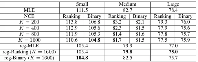
Table 1: Perplexity on the test set of Penn Treebank. We show performance for the ranking v.s. binary loss algorithms, with different values forK, and with/without regularization.

Figure 2: KL divergence between the true distribution and the estimated distribution.

ing the two NCE objectives. We use the unigram distribution as the negative sampling distribution and considerK = 200,400,800,1600.

The results on the test set are summarized in ta-ble 1. Similar patterns are observed on the vali-dation set (see Section A.2of the supplementary material). As shown in the table, the performance of NCE-ranking and NCE-binary improves as the number of negative examples increases, and fi-nally outperforms the MLE.

An interesting observation is, without regular-ization, the binary classification approach outper-forms both ranking and MLE. This suggests the model space (two-layer LSTMs) is rich enough as to approximately incorporate thex-dependent par-tition functionZ(✓;x), thus making the model

ap-proximately self-normalized. This motivates us to modify the ranking and MLE objectives by adding the following regularization term:

↵

n n

X

i=1

0 @log

0 @1

m m

X

j=1

exp⇣s¯(x(i),_ey(i,j);✓)⌘ 1 A

1 A

2

⇡↵EX

h

(logZ(x;✓))2i,

where ey(i,j),1  j  m are sampled from the noise distribution pN(·). This regularization

term promotes a constant partition function, that is Z(x;✓)_⇡1for allx_2X. In our experiments, we fixmto be 1/10 of the vocabulary size,K= 1600

and tune the regularization parameter↵. As shown

in the last three rows of the table, regularization significantly improves the performance of both the ranking approach and the MLE.

6 Conclusions

In this paper we have analyzed binary and rank-ing variants of NCE for estimation of conditional models p(y_|x;✓). The ranking-based variant is

consistent for a broader class of models than the binary-based algorithm. Both algorithms achieve Fisher efficiency as the number of negative exam-ples increases. Experiments show that both algo-rithms outperform MLE on a language modeling task. The ranking-based variant of NCE outper-forms the binary-based variant once a regularizer is introduced that encourages self-normalization.

Acknowledgments

References

Yoshua Bengio and Jean-S´ebastien Sen´ecal. 2008. Adaptive importance sampling to accelerate train-ing of a neural probabilistic language model. IEEE Transactions on Neural Networks, 19(4):713–722.

Adam L. Berger, Vincent J. Della Pietra, and Stephen A. Della Pietra. 1996. A maximum entropy ap-proach to natural language processing. Comput. Linguist., 22(1):39–71.

Thomas Shelburne Ferguson. 1996. A course in large sample theory, volume 49. Chapman & Hall Lon-don.

Michael U Gutmann and Aapo Hyv¨arinen. 2012. Noise-contrastive estimation of unnormalized sta-tistical models, with applications to natural image statistics. Journal of Machine Learning Research, 13(Feb):307–361.

Rafal Jozefowicz, Oriol Vinyals, Mike Schuster, Noam Shazeer, and Yonghui Wu. 2016. Exploring the limits of language modeling. arXiv preprint arXiv:1602.02410.

John D. Lafferty, Andrew McCallum, and Fernando C. N. Pereira. 2001. Conditional random fields: Probabilistic models for segmenting and labeling se-quence data. InProceedings of the Eighteenth Inter-national Conference on Machine Learning, ICML ’01, pages 282–289, San Francisco, CA, USA. Mor-gan Kaufmann Publishers Inc.

Omer Levy and Yoav Goldberg. 2014. Neural word embedding as implicit matrix factorization. In Pro-ceedings of the 27th International Conference on Neural Information Processing Systems - Volume 2, NIPS’14, pages 2177–2185, Cambridge, MA, USA. MIT Press.

Mitchell P Marcus, Mary Ann Marcinkiewicz, and Beatrice Santorini. 1993. Building a large annotated corpus of english: The penn treebank. Computa-tional linguistics, 19(2):313–330.

Tomas Mikolov, Ilya Sutskever, Kai Chen, Greg Cor-rado, and Jeffrey Dean. 2013. Distributed represen-tations of words and phrases and their composition-ality. InProceedings of the 26th International Conference on Neural Information Processing Systems -Volume 2, NIPS’13, pages 3111–3119, USA. Curran Associates Inc.

Andriy Mnih and Yee W Teh. 2012. A fast and simple algorithm for training neural probabilistic language models. In Proceedings of the 29th International Conference on Machine Learning (ICML-12), pages 1751–1758.

Zhilin Yang, Zihang Dai, Ruslan Salakhutdinov, and William W. Cohen. 2018. Breaking the softmax bottleneck: A high-rank RNN language model. In International Conference on Learning Representa-tions.