Combining Manual Rules and Supervised Learning for Hedge Cue and Scope Detection

Combining Manual Rules and Supervised Learning for Hedge Cue and

Scope Detection

Marek Rei Computer Laboratory University of Cambridge

United Kingdom

[email protected]

Ted Briscoe Computer Laboratory University of Cambridge

United Kingdom

[email protected]

Abstract

Hedge cues were detected using a super-vised Conditional Random Field (CRF) classifier exploiting features from the RASP parser. The CRF’s predictions were filtered using known cues and unseen in-stances were removed, increasing preci-sion while retaining recall. Rules for scope detection, based on the grammatical re-lations of the sentence and the part-of-speech tag of the cue, were manually-developed. However, another supervised CRF classifier was used to refine these pre-dictions. As a final step, scopes were con-structed from the classifier output using a small set of post-processing rules. Devel-opment of the system revealed a number of issues with the annotation scheme adopted by the organisers.

1 Introduction

Speculative or, more generally, “hedged” language is a way of weakening the strength of a statement. It is usually signalled by a word or phrase, called a hedge cue, which weakens some clauses or propo-sitions. These weakened portions of a sentence form the scope of the hedge cues.

Hedging is an important tool in scientific lan-guage allowing scientists to guide research be-yond the evidence without overstating what fol-lows from their work. Vincze et al. (2008) show that 19.44% of all sentences in the full papers of the BioScope corpus contain hedge cues. De-tecting these cues is potentially valuable for tasks such as scientific information extraction or liter-ature curation, as typically only definite informa-tion should be extracted and curated. Most work so far has been done on classifying entire text sentences as hedged or not, but this risks los-ing valuable information in (semi-)automated

sys-tems. More recent approaches attempt to find the specific parts of a text sentence that are hedged.

Here we describe a system that is designed to find hedge cues and their scopes in biomedical re-search papers. It works in three stages:

1. Detecting the cues using a token-level super-vised classifier.

2. Finding the scopes with a combination of manual rules and a second supervised token-level classifier.

3. Applying postprocessing rules to convert the token-level annotation into predictions about scope.

Parts of the system are similar to that of Morante and Daelemans (2009) — both make use of ma-chine learning to tag tokens as being in a cue or a scope. The most important differences are the use of manually defined rules and the inclusion of grammatical relations from a parser as critical fea-tures.

2 Data

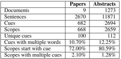
A revised version of the BioScope corpus (Vincze et al., 2008), containing annotation of cues and scopes, was provided as training data for the CoNLL-2010 shared task (Farkas et al., 2010). This includes 9 full papers and 1273 abstracts from biomedical research fields. A separate new set of full papers was released for evaluation as part of the task. Table 1 contains an overview of the training corpus statistics.

(1) provides an example sentence from the cor-pus illustrating the annotation provided for train-ing.

(2) shows the same sentence, representing cues with angle brackets and scopes with round brack-ets.

Papers Abstracts

Documents 9 1273

Sentences 2670 11871

Cues 682 2694

Scopes 668 2659

Unique cues 100 112

Cues with multiple words 10.70% 12.25% Scopes start with cue 72.00% 80.59% Scopes with multiple cues 2.10% 1.28%

Table 1: Training data statistics.

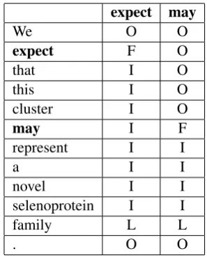
(1) <sentence id=“S1.166”>We<xcope id=“X1.166.2”><cue ref=“X1.166.2”

type=“speculation”>expect</cue>that this cluster

<xcope id=“X1.166.1”><cue ref=“X1.166.1” type=“speculation”>may</cue>represent a novel

selenoprotein

family</xcope></xcope>.</sentence>

(2) We (<expect>that this cluster (<may>represent a novel selenoprotein family)).

There are a number of conditions on the anno-tation that are imposed:

• Every cue has one scope.

• Every scope has one or more cues.

• The cue must be contained within its scope.

• Cues and scopes have to be continuous.

For development of the system, before the eval-uation data were released, we used 60% of the available corpus for training and 40% for testing. The results we give below measure the system per-formance on the evaluation data while using all of the training data to build the supervised clas-sifiers. The manually-developed rules are based on the 60% of the development data we originally reserved for training.

All of the training and test data sentences were tokenised and parsed using the RASP sys-tem (Briscoe et al., 2006). Multiple part-of-speech (POS) tag outputs were passed to the parser (to compensate for the high number of unseen words in biomedical text), retaining just the high-est ranked directed graph of grammatical relations (GRs). Each node in the graph represents a word token annotated with POS, lemma, and positional order information. In the case of parse failure the set of unconnected graphs returned by the highest-ranked spanning subanalyses for each sentence were retained.

3 Speculation cues

The hedge cues are found using a Conditional Random Field (CRF) (Lafferty et al., 2001) classi-fier, implemented using CRF++ 1_{. We chose the}

CRF model because we framed the task as one of token-level sequential tagging and CRFs are known to achieve state-of-the-art performance on related text classification tasks. Each word token is assigned one of the following tags:F(first word of a cue),I(inside a cue),L(last word of a cue), O(outside, not a cue), hereafter referred to as the FILO scheme.

The feature types used for classification are de-fined in terms of the grammatical relations output provided by the RASP system. We use binary fea-tures that indicate whether a word token is a head or a dependent in specific types of grammatical relation (GR). This distinguishes between differ-ent functions of the same word (when used as a subject, object, modifier, etc.). These features are combined with POS and lemma of the word to dis-tinguish between uses of different cues and cue types. We also utilise features for the lemma and POS of the 3 words before and after the current word.

The list of feature types for training the classi-fier is:

• string • lemma • part-of-speech

• broad part-of-speech • incoming GRs + POS • outgoing GRs + POS

• incoming GRs + POS + lemma • outgoing GRs + POS + lemma • lemma + POS + POS of next word

• lemma + POS + POS of previous word

• 3 previous lemma + POS combinations • 3 following lemma + POS combinations. Outgoing GRs are grammatical relations where the current word is the head, incoming GRs where it is the dependent.

The predictions from the classifier are com-pared to the list of known cues extracted from the training data; the longest possible match is marked as a cue. For example, the classifier could output the following tag sequence:

(3) This[O] indicates[F] that[O] these[O] two[O] lethal[O] mutations[O] . . .

indicates is classified as a cue but that is not. The list of known cues contains “indicates that” which matches this sentence, therefore the system prediction is:

(4) This<indicates that>these two lethal mutations . . .

Experiments in section 5.1 show that our sys-tem is not good at finding previously unseen cues. Lemma is the most important feature type for cue detection and when it is not available, there is not enough evidence to make good predictions. There-fore, we compare all system predictions to the list of known cues and if there is no match, they are removed. The detection of unseen hedge cues is a potential topic for future research.

4 Speculation scopes

We find a scope for each cue predicted in the pre-vious step. Each word token in the sentence is tagged with eitherF(first word of a scope),I (in-side a scope),L(last word of a scope) orO (out-side, not in a scope). Using our example sentence (2) the correct tagging is:

expect may

We O O

expect F O

that I O

this I O

cluster I O

may I F

represent I I

a I I

novel I I

selenoprotein I I

family L L

. O O

Table 2: Example of scope tagging.

If a cue contains multiple words, they are each processed separately and the predictions are later combined by postprocessing rules.

As the first step, manually written rules are ap-plied that find the scope based on GRs and POS tags. We refine these predictions using a second CRF classifier and further feature types extracted from the RASP system output. Finally, postpro-cessing rules are applied to convert the tagging se-quence into scopes. By default, the minimal scope returned is the cue itself.

4.1 Manual rules

Manual rules were constructed based on the de-velopment data and annotation guidelines. In the following rules and examples:

• “below” refers to nodes that are in the

sub-graph of GRs rooted in the current node.

• “parent” refers to the node that is the head of the current node in the directed, connected GR graph.

• “before” and “after” refer to word positions

in the text centered on the current node.

• “mark everything below” means mark all

nodes in the subgraph as being in the scope (i.e. tag as F/I/L as appropriate). However, the traversal of the graph is terminated when a text adjunct (TA) GR boundary or a word POS-tagged as a clause separator is found, since they often indicate the end of the scope.

The rules for finding the scope of a cue are trig-gered based on the generalised POS tag of the cue:

• Auxiliary — VM

Mark everything that is below the parent and after the cue.

If the parent verb is passive, mark everything below its subject (i.e. the dependent of the subj GR) before the cue.

• Verb — VV

Mark everything that is below the cue and af-ter the cue.

If cue isappearorseem, mark everything be-low subject before the cue.

If cue is passive, mark everything below sub-ject before the cue.

• Adjective — JJ

Find parent of cue. If there is no parent, the cue is used instead.

Mark everything that is below the parent and after the cue.

If parent is passive, mark everything below subject before the cue.

If cue is(un)likely and the next word is to, mark everything below subject before the cue.

• Adverb — RR

• Noun — NN

Find parent of cue. If there is no parent, the cue is used instead.

Mark everything that is below the parent and after the cue.

If parent is passive, mark everything below subject before the cue.

• Conjunction — CC

Mark everything below the conjunction. If the cue isorand there is another cueeither before, combine them together.

• “Whether” as a conjunction — CSW

Mark everything that is below the cue and af-ter the cue.

• Default — anything else

Mark everything that is below the parent and after the cue.

If parent verb is passive, mark everything be-low subject before the cue.

Either . . . or . . . is a frequent exception

contain-ing two separate cues that form a scontain-ingle scope. An additional rule combines these cues when they are found in the same sentence.

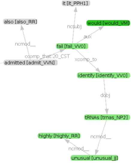
The partial GR graph for (5) is given in Figure 1 (with positional numbering suppressed for read-ability).

(5) Lobanov et al. thus developed a sensitive search method to deal with this problem, but they also admitted that it (<would>fail to identify highly unusual tRNAs).

Following the rules,wouldis identified as a cue word with the part-of-speech VM; this triggers the first rule in the list. The parent of would is fail since they are connected with a GR wherefailis the head. Everything that is belowfailin the GR graph and positioned afterwouldis marked as be-ing in the scope. Sincefailis not passive, the sub-jectitis left out. The final scope returned by the rule is then would fail to identify highly unusual

tRNAs.

4.2 Machine learning

The tagging sequence from the manual rules is used as input to a second CRF classifier, along with other feature types from RASP. The output of the classifier is a modified sequence of FILO tags.

The list of features for each token, used both alone and as sequences of 5-grams before and after the token, is:

Figure 1: Partial GR graph for sample sentence (5)

• tag from manual rules

• lemma

• POS

• is the token also the cue

• distance from the cue

• absolute distance from the cue • relative position to the cue

• are there brackets between the word and the cue

• is there any other punctuation between the word and the cue

• are there any special (clause ending) words

between the word and cue

• is the word in the GR subtree of the cue

• is the word in the GR subtree of the main verb • is the word in the GR subject subtree of the

main verb

Features of the current word, used in combina-tion with the POS sequence of the cue:

• POS

• distance from the cue

• absolute distance from the cue

• relative position to the cue

• is the word in the GR subtree of the cue • is the word in the GR subtree of the main verb

Additional features:

• GR paths between the word and the cue: full

path plus subpaths with up to 5 nodes

• GR paths in combination with the lemma se-quence of the cue

The scope of the hedge cue can often be found by tracking the sequence of grammatical relations in the GR graph of a sentence, as described by the manual rules. To allow the classifier to learn such regularities, we introduce the concept of a GR path.

Given that the sentence has a full parse and con-nected graph, we can find the shortest concon-nected path between any two words. We take the nected path between the word and the cue and con-vert it into a string representation to use it as a fea-ture value in the classifier. Path sections of differ-ent lengths allow the system to find both general and more specific patterns. POS tags are used as node values to abstract away from word tokens.

An example for the word unusual, using the graph from Figure 1, is given below. Five fea-tures representing paths with increasing lengths plus one feature containing the full path are ex-tracted.

(6) 1: VM

2: VM<–aux–VV0

3: VM<–aux–VV0–xcomp–>VV0

4: VM<–aux–VV0–xcomp–>VV0–dobj–>NP2

5: VM<–aux–VV0–xcomp–>VV0–dobj–>NP2–

ncmod–>JJ

6: VM<–aux–VV0–xcomp–>VV0–dobj–>NP2–

ncmod–>JJ

Line 1 shows the POS of the cuewould(VM). On line 2, this node is connected tofail(VV0) by an auxiliary GR type. More links are added until we reachunusual(JJ).

The presence of potential clause ending words, used by Morante and Daelemans (2009), is in-cluded as a feature type with values: whereas, but, although, nevertheless, notwithstanding, how-ever, consequently, hence, therefore, thus, instead, otherwise, alternatively, furthermore, moreover,

since.

4.3 Post-processing

If the cue contains multiple words, the tag se-quences have to be combined. This is done by overlapping the sequences and choosing the pre-ferred tag for each word, according to the hierar-chy F>L>I>O.

Next, scopes are constructed from tag se-quences using the following rules:

• Scope start point is the first token tagged as F before the cue. If none are found, the first word of the cue is used as the start point.

• Scope end point is the last token tagged as L after the cue. If none are found, look for tags I and F. If none are found, the last word of the cue is used as end point.

The scopes are further modified until none of the rules below return any updates:

• If the last token of the scope is punctuation,

move the endpoint before the token.

• If the last token is a closing bracket, move the scope endpoint before the opening bracket.

• If the last token is a number and it is not

pre-ceded by a capitalised word (e.g. Table 16), move the scope endpoint before the token. This is a heuristic rule to handle trailing ci-tations which are frequent in the training data and often misattached by the parser.

Finally, scopes are checked for partial overlap and any instances are corrected. For example, the system might return a faulty version (7) of the sen-tence (2) in which one scope is only partially con-tained within the other.

(7) We [<expect>that this cluster (<may>represent a novel] selenoprotein family).

This prediction cannot be represented within the format specified for the shared task and we were unable to find cases where such annotation would be needed. These scopes are modified by moving the end of the first scope to the end of the second scope. The example above would become:

(8) We [<expect>that this cluster (<may>represent a novel selenoprotein family)].

5 Results 5.1 Hedge cues

The results below are obtained using the scorers implemented by the organisers of the shared task.

As our baseline system, we use simple string matching. The list of known cues is collected from the training data and compared to the evaluation sentences. The longest possible match is always marked as a cue. ML1 to ML3 are variations of the system described in section 3. All available data, from papers and abstracts, were used to train the CRF classifier. ML1 uses the results of the classifier directly. The longest sequence of tokens tagged as being part of a cue is used to form the fi-nal prediction. ML2 incorporates the list of known cues, constructing a cue over the longest sequence of matching tokens where at least one token has been tagged as belonging to a cue. ML3 uses the list of known cues and also removes any predicted cues not seen in the training data.

Baseline ML1 ML2 ML3

Total cues 1047 1047 1047 1047

Predicted cues 3062 995 1006 995

Correctly

predicted cues 1018 785 810 810

Cue precision 0.332 0.789 0.805 0.814 Cue recall 0.972 0.750 0.774 0.774 Cue F-measure 0.495 0.769 0.789 0.793 Sentence

precision 0.413 0.831 0.831 0.838

Sentence recall 0.995 0.843 0.843 0.842 Sentence

F-measure 0.584 0.837 0.837 0.840

Table 3: Cue detection results.

The baseline system returns nearly all cues but since it matches every string, it also returns many false positives, resulting in low precision. ML1 delivers more realistic predictions and increases precision to 0.79. This illustrates how the use of a word as a hedge cue depends on its context and not only on the word itself. ML2 incorporates known cues and increases both precision and recall. ML3 removes any unseen cue predictions further im-proving precision. This shows the system is un-able to accurately predict cues that have not been included in the training data.

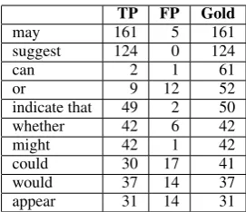
Table 4 lists the ten most common cues in the test data and the number of cues found by the ML3 system.

In the cases ofmayandsuggest, which are also the most common cues in the development data, the system finds all the correct instances. Can andorare not detected as accurately because they are both common words that in most cases are

TP FP Gold

may 161 5 161

suggest 124 0 124

can 2 1 61

or 9 12 52

indicate that 49 2 50

whether 42 6 42

might 42 1 42

could 30 17 41

would 37 14 37

appear 31 14 31

Table 4: True and false positives of the ten most common cues in the evaluation data, using ML3 system.

not functioning as hedges. For example, there are 1215 occurrences of or in the training data and only 146 of them are hedge cues;canis a cue in 64 out of 506 instances. We have not found any ex-tractable features that reliably distinguish between the different uses of these words.

5.2 Hedge scopes

A scope is counted as correct if it has the correct beginning and end points in the sentence and is associated with the correct cues. Scope prediction systems take cues as input, therefore we present two separate evaluations – one with gold standard cues and the other with cues predicted by the ML3 system from section 4.

The baseline system looks at each cue and marks a scope from the beginning of the cue to the end of the sentence, excluding the full stop. The system using manual rules applies a rule for each cue to find its scope, as described in section 4.1. The POS tag of the cue is used to decide which rule should be used and the GRs determine the scope.

The final system uses the result from the manual rules to derive features, adds various further fea-tures from the parser and trains a CRF classifier to refine the predictions.

We hypothesized that the speculative sentences in abstracts may differ from the ones in full papers and a 10-fold cross-validation of the development data supported this intuition. Therefore, the orig-inal system (CRF1) only used data from the full papers to train the scope detection classifier. We present here also the system trained on all of the available data (CRF2).

Post-processing rules are applied equally to all of these systems.

Baseline Manual

rules Manualrules + CRF1

Manual rules + CRF2

Total scopes 1033 1033 1033 1033

Predicted 1047 1035 1035 1035

Correctly

predicted 596 661 686 683

Precision 0.569 0.639 0.663 0.660

Recall 0.577 0.640 0.664 0.661

F-measure 0.573 0.639 0.663 0.661

Table 5: Scope detection results using gold stan-dard cues.

Baseline Manual

rules Manualrules + CRF1

Manual rules + CRF2

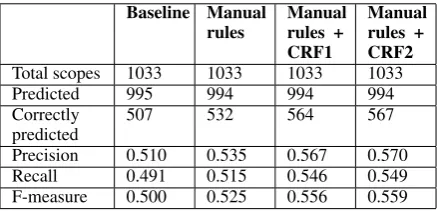
Total scopes 1033 1033 1033 1033

Predicted 995 994 994 994

Correctly

predicted 507 532 564 567

Precision 0.510 0.535 0.567 0.570

Recall 0.491 0.515 0.546 0.549

F-measure 0.500 0.525 0.556 0.559

Table 6: Scope detection results using predicted cues.

It does not use any grammatical or lexical know-ledge apart from the cue and yet it delivers an F-score of 0.50 with predicted and 0.57 with gold standard cues.

Manual rules are essentially a more fine-grained version of the baseline. Instead of a single rule, one of 8 possible rules is selected based on the POS tag of the cue. This improves the results, increasing the F-score to 0.53 with predicted and 0.64 with gold standard cues. The improvement suggests that the POS tag of a cue is a good indi-cator of how it behaves in the sentence.

Error analysis showed that 35% of faulty scopes were due to incorrect or unconnected GR graphs output by the parser, and 65% due to exceptions that the rules do not cover. An example of an ex-ception, the braces { } showing the scopes

pre-dicted by the rules, is given in (9).

(9) Contamination is{(<probably>below 1%)}, which is{(<likely>lower than the contamination rate of the positive dataset) as discussed in 47}.

as discussed in 47 is a modifier of the clause

which is usually included in the scope but in this case should be left out.

Finally, the last system combines features from the rule-based system with features from RASP to train a second classifier and improves our results further, reaching 0.56 with predicted cues.

Inclusion of the abstracts as training data gave a small improvement with predicted cues but not with gold standard cues. It is part of future work to determine if and how the use of hedges differs across text sources.

6 Annotation scheme

During analysis of the data, several examples were found that could not be correctly annotated due to the restrictions of the markup. This leads us to believe that the current rules for annotation might not be best suited to handle complex constructions containing hedged text.

Most importantly, the requirement for the hedge scope to be continuous over the surface form of text sentence does not work for some examples drawn from the development data. In (10) below it is uncertain whether fat body disintegration is independent of the AdoR. In contrast, it is stated with certainty that fat body disintegration is pro-moted by action of the hemocytes, yet the latter assertion is included in the scope to keep it contin-uous.

(10) (The block of pupariation<appears>to involve signaling through the adenosine receptor ( AdoR )) , but (fat body disintegration , which is promoted by action of the hemocytes ,<seems>to be independent of the AdoR) .

Similarly, according to the guidelines, the sub-ject of be likely should be included in its scope, as shown in example (11). In sentence (12), how-ever, the subjectthis phenomenonis separated by two non-speculative clauses and is therefore left out of the scope.

(11) Some predictors make use of the observation that (neighboring genes whose relative location is conserved across several prokaryotic organisms are

<likely>to interact).

(12) This phenomenon, which is independent of tumour necrosis factor, is associated with HIV replication, and (is thus<likely>to explain at least in part the

perpetuation of HIV infection in monocytes).

In (13), arguably, there is no hedging as the sen-tence precisely describes a statistical technique for predicting interaction given an assumption.

(13) More recently, other groups have come up with sophisticated statistical methods to estimate

(<putatively>interacting domain pairs), based on the (<assumption>of domain reusability).

hedge scope in terms of sets of semantic proposi-tions recovered from a logical semantic represen-tation of the text, in which anaphora, word sense, and entailments had been resolved.

7 Related work

Most of the previous work has been done on classi-fying sentences as hedged or not, rather than find-ing the scope of the hedge.

The first linguistically and computationally mo-tivated study of hedging in biomedical texts is Light et al. (2004). They present an analysis of the problem based on Medline abstracts and construct an initial experiment for automated classification.

Medlock and Briscoe (2007) propose a weakly supervised machine learning approach to the hedge classification problem. They construct a classifier with single words as features and use a small amount of seed data to bootstrap the system, achieving the precision/recall break-even point (BEP) of 0.76. Szarvas (2008) extends this work by introducing bigrams and trigrams as fea-ture types, improving feafea-ture selection and us-ing external data sources to construct lists of cue words, achieving a BEP of 0.85.

Kilicoglu and Bergler (2008) apply a combina-tion of lexical and syntactic methods, improving on previous results and showing that quantifying the strength of a hedge can be beneficial for clas-sification of speculative sentences.

Vincze et al. (2008) created a publicly available annotated corpus of biomedical papers, abstracts and clinical data called BioScope, parts of which were also used as training data for the CoNLL10 shared task, building on the dataset and annota-tion scheme used for evaluaannota-tion by Medlock and Briscoe (2007).

Morante and Daelemans (2009) use the Bio-Scope corpus to approach the problem of identify-ing cues and scopes via supervised machine learn-ing. They train a selection of classifiers to tag each word and combine the results with a final classi-fier, finding 65.6% of the scopes in abstracts and 35.9% of the scopes in papers.

8 Conclusions

We have shown that the GRs output by the RASP system can be effectively used as features for de-tecting cues in a supervised classifier and also as the basis for manual rules and features for scope detection. We demonstrated that a small

num-ber of manual rules can provide competitive re-sults, but that these can be further improved using machine learning techniques and post-processing rules. The generally low ceiling for the scope de-tection results demonstrates the difficulty of both annotating and detecting the hedge scopes in terms of surface sentential forms.

Future work could usefully be directed at im-proving performance on unseen cue detection and on learning rules of the same form as those de-veloped manually from annotated training data. However, perhaps the most pressing issue is that of establishing the best possible annotation and con-sequent definition of the scope detection task.

References

Ted Briscoe, John Carroll, and Rebecca Watson. 2006. The second release of the RASP system. In Pro-ceedings of the COLING/ACL 2006 on Interactive Presentation Sessions.

Rich´ard Farkas, Veronika Vincze, Gy¨orgy M´ora, J´anos Csirik, and Gy¨orgy Szarvas. 2010. The CoNLL-2010 Shared Task: Learning to Detect Hedges and their Scope in Natural Language Text. In Proceed-ings of the Fourteenth Conference on Computational Natural Language Learning (CoNLL-2010): Shared Task, pages 1–12.

Halil Kilicoglu and Sabine Bergler. 2008. Recogniz-ing speculative language in biomedical research ar-ticles: a linguistically motivated perspective. BMC Bioinformatics, 9 Suppl 11.

John Lafferty, Andrew McCallum, and Fernando Pereira. 2001. Conditional random fields: Prob-abilistic models for segmenting and labeling se-quence data. InProceedings of ICML 2001. Marc Light, Xin Y. Qiu, and Padmini Srinivasan. 2004.

The language of bioscience: Facts, speculations, and statements in between. In Proceedings of BioLink 2004.

Ben Medlock and Ted Briscoe. 2007. Weakly super-vised learning for hedge classification in scientific literature. InProceedings of ACL 2007.

Roser Morante and Walter Daelemans. 2009. Learn-ing the scope of hedge cues in biomedical texts. In

Proceedings of the Workshop on BioNLP.

Gy¨orgy Szarvas. 2008. Hedge classification in biomedical texts with a weakly supervised selection of keywords. InProceedings of ACL 2008.