Abstract
—
Efficient discovery of maximal frequent itemsets (MFI) in large databases is an important problem in data mining. Many approaches have been suggested such as sequential mining for maximal frequent itemsets or searching for all frequent itemsets in parallel. So far, those approaches are still not genuinely effective to mine extremely large databases. In this work we propose a parallel method for mining MFI using PC clusters, exploiting their relationships between MFI locally found in the cluster nodes and the global MFI, and derive a top-down mechanism which produces fewer candidates and substantially reduce the number of messages passed among PCs. We also provide a clustering-based method to partition the database to achieve a good balance of loading among the nodes.Evaluations on our method have been performed using both synthetic and real databases. Empirical results show that our method has a superior performance over the direct application of a typical sequential MFI mining algorithm.
Index Terms—
Parallel Data Mining, Maximal Frequent Itemsets,Partition, PC Cluster
I. I
NTRODUCTIONMining frequent itemsets [1][5][13] is a fundamental and essential problem in many data mining applications, such as association rule discovery, correlations detection and multidimensional pattern identification. The framework of mining frequent itemsets was originally proposed by Agrawal et al. [1].
Let I = {i1, i2, …, in} be a set of literals, called items and n is
considered the dimensionality of the item. Let D be a set of transactions, where each transaction T is a set of items such as T⊆I.
A transaction T is said to contain X, a set of items in I, if X⊆T. An itemset X is said to be frequent if its support s is greater than or equal to given minimum support call thresholdσ. A frequent itemset М is considered maximal if there is no other frequent itemset that is superset of М. Consequently, any subset of a maximal pattern is a frequent pattern. Discovering all maximal patterns effortlessly yields the complete set of frequent patterns.
Many algorithms of the proposed frequent itemset mining are variants of Apriori [1], which employ a bottom-up, breadth-first search that enumerates every single frequent itemset. In many applications (especially in dense data), enumerating all possible 2m−2 subsets of a m length pattern (m can easily be 30 or 40 or longer) is computationally unfeasible. Thus, mining maximal frequent itemset (MFI) attracts much attention in recent years.
Manuscript received December 10, 2007.
Vong Chan Veng, Terry is with the Macau University of Science and Technology, Macao S.A.R (phone: 853-88972089; email: [email protected])
MaxMiner [4], DepthProject [3], GenMax [9] and MAFIA [6] are well-known solutions in mining MFI.
As databases become larger, sequential data mining algorithms have become an unacceptable solution. Thus, parallel mining may deliver an effective solution on huge database. Parallel approaches for mining frequent itemsets are mainly based on two paradigms, Count Distribution and Data Distribution, all inherit Apriori’s level-wise processing style. Algorithms that belong to Count Distribution include CD [2], PDM [14] and FPM [8]. Algorithms which belong to Data Distribution include DD [2], IDD [10] and HPA [15].
As far as we know, most of the proposed parallel mining algorithms are well tuned for discovering frequent itemsets rather than maximal frequent itemsets. These methods are not easily extended to handle the maximal frequent itemsets. Therefore we try to solve the problem from another way. That is, local MFI on each node is generated first, and then the relationships between local MFIs and global MFIare explored to generate candidates with a top-down manner. These relationships also guide us to partition databases in a special way, which not only achieves a good balance in loading among the nodes in the cluster but also produces fewer candidates. This in turn makes our algorithm faster both in counting and in sending fewer messages among nodes. Our contributions can be summarized as follows.
We introduce the first approach of parallel mining MFIon PC clusters, DMFI, which can be easily integrated with any available sequential MFImining algorithm. It greatly reduces the number of candidates by following a top-down candidate generation approach.
We have shown some interesting relationships between locally found MFI and global MFI which enable us to generate global MFIfrom local MFIs.
We also propose an efficient and effective clustering based database partitioning algorithm to partition the database into the cluster nodes, which in general can help to balance the workload for each node in the cluster.
We have evaluated our approach using both synthetic and real databases. The results show that our approach is efficient and effective.
The rest parts of paper are organized as follows: In section 2, we discuss the relationships between locally found MFI and global
MFI. Our algorithm for parallel mining of MFIis also presented in this section. In section 3, we discuss how to effectively partition database into the cluster nodes. The performance evaluation is presented in Section 4. Finally, Section 5 concludes the paper and presents some of the possible future works.
II. M
ININGOF
THE MAXIMAL FREQUENT ITEMSETS
In this section, we first elaborate the relationships between local
MFIin each cluster nodes and global MFI, which essentially enable us to design our method, DMFI.
Parallel Mining of Maximal Frequent Itemsets in
PC Clusters
A. Relationships between Local and Global MFI
Let Ddenotes a database, which is partitioned into d1, d2,..., dn parts
for n nodes respectively. Let MFIi, Fiand Iibe the sets of maximal frequent itemsets, frequent but not maximal itemsets and infrequent itemsets in the ith PC cluster node respectively. Let MFI, Fand Ibe
the sets of maximal frequent itemsets, frequent but not maximal itemsets and infrequent itemsets in D. Obviously, MFIi, Fi and Ii only carry local information, but MFI, F and Irepresent the global information.
Given an itemset q can only be MFIor F or Ion the each node. Therefore, nnodes imply 3n combinations of a maximal frequent itemset can be produced. However, it is easy to classify these combinations into 7 cases:
(1) q is local maximal frequent in all nodes. (2) q is local frequent in all nodes but not maximal. (3) q is infrequent in all nodes.
(4) q is local maximal in some of nodes, but infrequent in others. (5) q is local maximal in some of nodes, but frequent in others. (6) qis local frequent in some of nodes, but infrequent in others. (7) q is local maximal frequent, frequent and infrequent in all nodes.
The case 3 can be skipped because itemset q is infrequent in all nodes. It is no doubt about case 1, itemset q must be global maximal frequent. For case 4, 5 and 7, itemset qis local maximal frequent in at least one node, when the minimum support of itemset q in whole database is greater than threshold, then itemset q is also global maximal frequent.
After checking those cases, itemsets in MFIx that are globally maximal frequent partially composing MFI. In addition, we use
loser to denote those itemsets in MFIx, which turn out to be not in
MFI. When loser is empty, that means no more itemsets can join global MFI, our algorithm can be stopped. Otherwise, the case 2 and 6 must be considered, they may turn out to be a global maximal frequent itemset. The following shows how we can determine if a frequent itemset qfound locally in the cluster nodes is a member of
MFI.
In case 2 and 6, itemset q is global maximal frequent itemset if and only if it doesn’t exist a superset in global MFI and its support in whole database is greater than threshold.
B. Algorithm DMFI
/* Input D, n, threshold*/ /* Output MFI*/
1). divide D into D1, D2, ..., Dn
2). Run available algorithm on each Dito get MFIi 3). MFI=MFI1∩MFI2 ∩ ... ∩MFIn
4). MFI1 ...n = MFI1 ...n - MFI 5). loser = ∅
6). for each d∈ MFI1 ...n
7). . . sup(d) = sup1(d) + sup2(d) + ... + supn(d)
8). . . . if sup(d)≥ threshold
9). . . then MFI = MFI {d}
10). . . else loser = loser {d}
11). maxsize now stores the length of the longest itemset in loser
12). while( loser≠∅ ) 13). . candidate = ∅
14). . for each q ∈ loser with |q| = maxsize
15). . . Z = {v|v ⊂ q, |v| + 1 = |q|} 16). . . candidate = candidate Z
17). . while (candidate≠∅ ) 18). . . for each q in candidate
19). . . . if q is a subset of some itemset(s) in MFI
20). . . then remove q from candidate
21). . send candidate to n PCs to do frequency counting
22). . get frequencies for candidate from each PC 23). . for each c ∈ candidate
24). . . sup(c) = sup1(c) + sup2(c) + ... + supn(c)
25). . . . if c.sup ≥ threshold
26). . . then MFI = MFI {c}
27). . . . else loser = loser {c}
28). . maxsize = maxsize −1
Figure 1.The DMFI Algorithm
In DMFI, candidates are generated and organized by their lengths. For each length, communication between server and clients is carried out for requesting candidate’s frequencies counting (from server to clients) and for answering frequency for each candidate (from clients to server). In real implementation, one client can play the role of server.
C. Subset Checking
We can skip the counting of an itemset if it is already a subset of a member in MFI. Therefore, besides frequency counting, subset checking is one of the most time consuming task in MFImining. In [9], subset checking is already embedded in the process of mining
MFIwith high efficiency. In our method, after using any available algorithm to discover all MFIi, we follow a top-down mechanism to generate candidate for validation, therefore the idea used in [9] cannot be applied here any more.
We construct a bit matrix to do subset checking, with the number of rows is equal to the number of items in the database, while the number of column is equal to the current size of MFI. In this matrix, each itemset in MFI is encoded in a column, where the ith bit is set to
”1” if the related item occurs in it or ”0” otherwise. Given an itemset
q = {2, 4, 5}for subset checking, we can AND the 2nd, the 4th and the
5th rows in the bit matrix and see whether there is a bit ”1” in the
result. If we find one that means the itemset is a subset of at least one member in MFI, and the checking can be stopped. Otherwise, it is not a subset of any itemsets in MFI.
III. D
ATABASEP
ARTITIONINGIn this section, we first present the relationship between commonality of FI and MFI, and then show a clustering based partitioning method.
Definition 2 The size of MFI after Case (1) over the final size of MFI is defined as the commonality of MFI.
Definition 3 The size of FI1 ∩ FI2∩ ... ∩ FIn over the size of FI is
defined as the commonality of FI.
Definition 4 The size of MFI after Case (1) and (4) over the final size of MFI is defined as MFI coverage.
A. Relationship between Commonality of FI and MFI
It is easy to see the performance of our algorithm is dominated by
loser, the smaller the loserin size, the better the performance. A smaller initialized loseris a good starting point to lead to a smaller
loser. In DMFI, the initial size of loser is controlled by the commonality of MFI: the larger the commonality of MFI, the smaller the initial size of loser. But how to achieve this?
As we know, maximal frequent itemsets represent a higher level information summary compared with frequent itemsets. And intuitively, high commonality of FI leads to high commonality of
MFI. Therefore we resort to seeking method that brings us high FI
rather than MFI.
acceptable probability for case where frequency error rate exceeds our expectation. For example, if an acceptable probability of 0.001 for an error rate of more than 0.001, then a 50,000 sampling size is sufficient. Obviously, the formula in [16] tells us a good sampling size can unveil most of the real frequent itemsets in database with high accuracy in their frequencies. But we interpret sampling in another way, namely, we get n samples from the database, where the size of each sample is |D|/n. Because each partition is an essential sample of the database. If the size of sampling is large enough according to [16], the commonality among frequent itemsets discovered in each partition should be high, which implies a high commonality among the maximal frequent itemsets in each partition, so that we may have a loser with smaller size.
Based on [16], if the size of each partition is large enough, we can derive a high commonality of FI. In fact, this is verified by our experiments. We notice that the commonality of FI is always above 95% in all FI computable experiments, and many of them even reach 99%. However, the related commonalities of MFI do not show the same optimistic result. It can drop down to 40% in one case. Why does this happen? This is mainly because MFI represents a much higher level of information summary compared against FI. Let us see an example, there are two sets FI1 =
{AB,AC,AD,BC,BD,CD,ABC,ABD,ACD,BCD,ABCD} and FI2 = {AB,AC,AD,BC,BD, CD,ABC,ABD,ACD}. BCD, ABCD are missed from FI2. MFI1 = {ABCD}and MFI2 = {ABC, ABD, ACD}, they are
completely different. In general, given X% commonality of FI, we should not expect the same X% but a lower, say Y % commonality of
MFI. Till now, we have not traced how to compute the difference between X% and Y %.
At the current stage, we can only conclude that increasing commonality of FI will give us a relatively high commonality of
MFI. Because low commonality between FIi, 1 ≤ i ≤ n always leads to lower commonality of MFI. Based on the previous discussion, we should divide the database in a special way such that the commonality among FIis is as high as possible. One way to achieve this is to distribute similar transactions to different PCs, so that they might generate roughly the same set of frequent itemsets in each PC. We have tested several ways to do the partitioning and have designed a clustering based partitioning method, which always brings us a smaller size loser compared with several other obvious partitioning methods.
B. Clustering Based Partitioning
Previous discussion points out that we can assign similar transactions into different PCs, so that different PC can generate FI
with high commonality. Our clustering based partitioning method follows this direction. Namely, transactions are grouped into clusters, where transactions in each cluster are similar, *so that they are distributed to different PCs. As an extension of K-means, our method is a three steps procedure. In the first step, a sample S is drawn the database, and then the distance between each pair of transactions in S is computed. The pair of transactions that have the largest distance become two seeds. After that, we iteratively choose a transaction as a new seed until we have K seeds. The chosen seed should maximize the sum of distance to all available seeds. The second step is also a loop process, it runs until the K seeds are stable in two consecutive iterations. In the each iteration, after assigning each transaction to its nearest seed, we have K clusters. Now, seed of each cluster is replaced by the transaction in this cluster so that the sum of distance between the new seed and all other transaction in this cluster is minimized. The third step is the real partitioning step based on K seeds get in the second step. For all clusters, we divide the distance range [0, 1] into M consecutive slots with equal
width, and associate each slot with an index indicating which partition will accept the next transaction falling in this slot. All indices are initialized to one, and increase by one after each assignment. If it is equals to the number of PCs, then it is back to one again. Now we can sequentially scan the database, after reading a transaction, it is assigned to the nearest seed and is dropped into a slot, related index tells us which partition this transaction should be distributed to.
[image:3.612.338.509.274.375.2]Workload balance is a hard problem in parallel processing. In our case, the workload is essentially the time used on counting frequencies of candidates. This is determined by three factors: the number of transactions, number of candidates and the average length of candidates in each PC. It is easy to see the number of transactions distributed to each PC is roughly the same by our method. Further because similar transactions are distributed into different PCs, therefore candidates produced in each PC should be similar, which makes us believe the number of candidates and the average length of them in each PC should be close. Under this condition, the workload distributed among different PCs should be balanced. This is verified by our experimental results.
Figure 2.Clustering Based Partition
Let us see an example in Figure 2. Here, we have one cluster with seed C. By scanning database, the 1st, 4th and 5th transactions drop in
the second distance slot of C one by one. Therefore, they are distributed to PC1, PC2 and PC3 respectively. If there is one more transaction falling in the same slot later on, itwill be assigned to PC1 again.
Selection of K
As a variant of K-means, our method also faces the difficult question, what value should K be? In [7], a new two-phase sampling based algorithm for discovering frequent itemsets was implemented. The foundation of the method was simple; a good sample should produce accurate frequency information for all items as possible. We extend the idea a little bit to fit our problem, namely, a good K should make the sum of frequency-difference among items in different partitions as small as possible. More formally, we hope to minimize the following formula. Here P denotes the number of partitions, supk(Ix) denotes the support of the xth item in I on the kth
partition.
∑ ∑ ∑
= = + =
=
−
Pk P
k j
I x
x
x j x
k
I
I
1 1 | |
1
|
)
(
sup
)
(
sup
|
IV.
EXPERIMENTAL RESULTSIn this section we present the results of the performance evaluation of DMFI in PC cluster and compare its performance against GenMax running on a single PC. Both synthetic and real databases are used. Because of the limitation of resources, we can only test our method on at most 4 PCs.
Two synthetic databases were created using the data generator from IBM Almaden denoted by T10I4D1000K and T40I10D200K, where there were 1000 items. The two real databases are Chess which contains 3196 transactions with 75 items and Mushroom which contains 8124 transactions with 130 items. For each database, experiments are carried out with three supporting thresholds on 1, 2, 3 and 4 PCs respectively. All PCs are using Windows XP as the OS with Intel P4 2.4GHz and 512MB main memory. Java 5.0 SE is the programming language.
A. Tests on Real Data
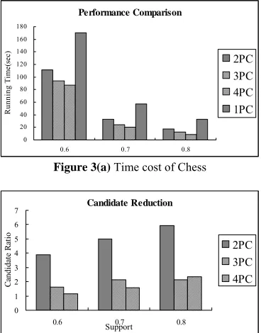
Notice that the two real databases contain only thousands of transactions, counting on them is extremely fast. Therefore, we enlarge the sizes of Mushroom and Chess to 200 times and 400 times of their original sizes respectively. The enlarging process is simple, read a database in and write it out to another file 200 or 400 times. Figure 3 shows the experimental results on Chess and Mushroom. Here (a) and (c) indicate the time cost while (b) and (d) present the candidate ratio, which is computed as dividing number of candidates on one PC by the number of candidates in DMFI that really need to be counted on each PC.
There are two observations from these two figures, (1) as we expected, when the number of PC increases, the time cost reduces accordingly and both reach the best performance with 4 PCs. With 4 PCs, the speed up of Chess is ranging from 2 to 3, while Mushroom ranges from 3 to 3.6. (2) As the number of PC increases, the number of candidate increases accordingly. This is mainly because the commonality of MFI reduces along with the number of PC increases, which produces a loser with larger initial size. At the worst case, the candidate ratio approaches to 1 in Chess. However, candidate ratios for mushroom are pretty good. We believe this is caused by our clustering-based partitioning method, which can not fully capture the characteristics of Chess data.
Performance Comparison
0 20 40 60 80 100 120 140 160 180
0.6 0.7 0.8
R
unning T
im
e(
se
c) 2PC
3PC 4PC 1PC
Figure 3(a) Time cost of Chess
Candidate Reduction
0 1 2 3 4 5 6 7
0.6 Support0.7 0.8
C
andi
da
te
R
at
io
2PC 3PC 4PC
Figure 3(b) Candidate Ratio of Chess
Performance Comparison
0 20 40 60 80 100 120
0.1 0.2 0.3
R
unn
ing T
im
e(
se
c) 2PC
3PC 4PC 1PC
Figure 3(c) Time cost of Mushroom
Candidate Reduction
0 1 2 3 4 5 6 7 8 9 10
0.1 0.2 0.3
Support
C
andida
te
R
ati
o
2PC 3PC 4PC
Figure 3(d) Candidate Ratio of Mushroom
B. Tests on Synthetic Data
Figure 4 shows the experimental results on T10I4D1000K and T40I10D200K.
Performance Comparison
0 100 200 300 400 500 600 700 800 900 1000
0.0005 0.001 0.005
R
unning T
im
e(
se
c)
2PC 3PC 4PC 1PC
Figure 4(a)Time cost of T10I4D1000K
Candidate Reduction
0 50 100 150 200 250 300 350 400 450
0.0005 0.001 0.005
Support
C
andida
te
R
ati
o
2PC 3PC 4PC
[image:4.612.331.519.45.299.2] [image:4.612.331.520.366.618.2] [image:4.612.93.277.483.718.2]Performance Comparison 0 5 10 15 20 25 30 35 40 45 50
0.02 0.05 0.1
R unning T im e( se c) 2PC 3PC 4PC 1PC
Figure 4(c) Time cost of T40I10D200K
Candidate Reduction 0 500 1000 1500 2000 2500 3000 3500 4000 4500
0.02 0.05 0.1
Support C andi da te R at io 2PC 3PC 4PC
Figure 4(d) Candidate Ratio of T40I10D200K
The general trends occur in real database appear again with one exception, that is the candidate ratios are very good in all presented cases. The major reason behind this is synthetic data is far more uniform compared against real database.
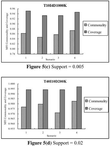
C. Varying Partitioning Methods
In this set of experiments, we test the effectiveness of different partitioning methods in terms of MFI commonality and coverage. Figure 5 shows four different database partitioning methods on real and synthetic databases with 2PCs. The four methods are: 1)random distribution, 2)sort all transactions by all of their items in increasing order and then randomly distribute, 3)sort all transactions by half of their items in increasing order and then randomly distribute, 4)our clustering-based method. Chess 0.00 0.10 0.20 0.30 0.40 0.50 0.60
1 2 3 4
Scenario M FI C om m ona lit y a nd C ove ra ge Commonality Coverage
Figure 5(a) Support = 0.6
Mushroom 0.000 0.100 0.200 0.300 0.400 0.500 0.600 0.700 0.800 0.900 1.000
1 2 3 4
Scenario M FI C omm ona lit y a nd C ove ra ge Commonality Coverage
Figure 5(b) Support = 0.1
T10I4D1000K 0.78 0.80 0.82 0.84 0.86 0.88 0.90 0.92 0.94 0.96
1 2 Scenario 3 4
M FI C om m ona lit y a nd C ove ra ge Commonality Coverage
Figure 5(c) Support = 0.005
T40I10D200K 0.955 0.960 0.965 0.970 0.975 0.980 0.985 0.990 0.995 1.000
1 2 3 4
Scenario M FI C om m ona lit y a nd C ove ra ge Commonality Coverage
Figure 5(d) Support = 0.02
Except performing a little bit worse than method 1) in coverage of case T10I4D1000K, our method outperforms all other methods in all other cases. Although it performs well in all three other cases, randomly distribution performs the worst for Chess, no commonality of MFI at all. As a consequence of high candidate ratio depicted in Figure 5 (b) and (d), it is not strange to see extremely high commonality and coverage of MFI for synthetic databases. They can even approach to 99.5%.
D. Commonality of FI and MFI
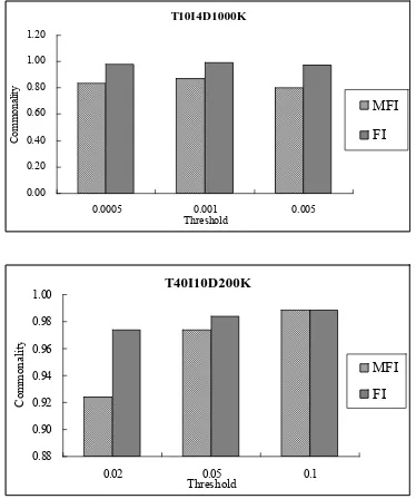
As we have not discovered the quantitative relationship on commonality between FI and MFI, we can only show some comparisons here. Figure 6 shows the commonality of MFI and FI
on real and synthetic databases in 2 PCs respectively. It is easy to see the commonality of FI is always very high, above 95%; however, the related commonality of MFI is not always so optimistic. Chess 0.00 0.20 0.40 0.60 0.80 1.00 1.20
0.6 0.7 0.8 Threshold Co m m on alit y MFI FI Mushroom 0.00 0.20 0.40 0.60 0.80 1.00 1.20
[image:5.612.94.277.46.308.2] [image:5.612.334.520.48.295.2] [image:5.612.91.279.478.716.2] [image:5.612.334.518.497.722.2]T10I4D1000K
0.00 0.20 0.40 0.60 0.80 1.00 1.20
0.0005 0.001 0.005 Threshold
C
ommo
na
lit
y
MFI
FI
T40I10D200K
0.88 0.90 0.92 0.94 0.96 0.98 1.00
0.02 0.05 0.1 Threshold
Co
m
m
on
alit
y
[image:6.612.91.278.49.273.2]MFI FI
Figure 6 MFI and FI Commonalities of Real and Synthetic Databases in 2 PCs
E. Remark on workload balance and communication cost
In all above experiments, we record the average candidate length and number of candidate in each PC and find out that they are close in all the cases. We also record the time used for communication, and notice that it is always less than 5% of the total time
V. CONCLUSIONS
Parallel mining of frequent itemsets have already been extensively studied with many efficient algorithms proposed. However, directly apply those methods in discovering maximal frequent itemsets is not easy because a global maximal frequent itemset may not be locally maximal frequent in at least one partition of database. In this paper, we follow another approach, database is partitioned in a special way, such that the commonality of local discovered maximal frequent itemsets from different partitions is maximized as possible. For those itemsets that do not contribute to the commonality, they are decomposed to produce candidates in a top-down manner rather than a general bottom-up manner extensively used in other approaches for mining frequent itemsets. The success of our algorithm is determined by whether we can partition the database good enough to achieve high commonality of locally discovered maximal frequent itemsets. To solve this problem, we designed a simple, but effective clustering base method, for which the effectiveness has been experimentally verified by both synthetic and real data.
One unsolved problem is the relationship between commonality of frequent itemsets and maximal itemsets. If it is uncovered, we might be able to get better partitioning method. Another direction is to unveil the relationship between MFI and partitions directly, rather than relying on FI to do partitioning. It is easy to see the server might become the bottle neck as more clients are involved. We will try totackle this by using more than one server and overlapping the counting process with communication period in server(s).
VI. REFERENCES
[1] R. Agrawal and R. Srikant. Fast algorithms for mining association rules. In Proceedings of International Conference on Very Large Data Bases, 1994.
[2] R. Agrawal, and J. C. Shafer. Parallel Mining of Association Rules IEEE Transaction on Knowledge and Data Engineering, Vol 8, 1996.
[3] R. C. Agarwal, C. C. Aggarwal and V. V. V. Prasad A tree projection algorithm for generation of frequent item sets. Journal of Parallel and Distributed Computing, Vol. 61, No. 3, 2001. [4] R.J. Bayardo. Efficiently Mining Long Patterns from Databases.
In Proceedings of ACM-SIGMOD International Conference on Management of Data, 1998.
[5] S. Brin, R. Motwani, J. Ullman, and S. Tsur. Dynamic Itemset Counting and Implication Rules for Market Basket Data. In Proceedings of ACM-SIGMOD International Conference on Management of Data, 1997.
[6] D. Burdick, M. Calimlim, J. Flannick, J. Gehrke and T. Yiu. MAFIA: a maximal frequent itemset algorithm IEEE Transaction on Knowledge and Data Engineering, Vol. 17, No. 11, 2005. [7] B. Chen, P. Haas and P. Scheuermann. A New Two-Phase Sampling Based Algorithm for Discovering Association Rules. In Proceedings of ACM-SIGKDD Conference, 2002.
[8] D. W. Cheung, S.D. Lee and Y. Xiao. Effect of Data Skewness and Workload Balance in Parallel Data Mining. IEEE Transaction on Knowledge and Data Engineering, Vol 14, May, 2002. [9] K. Gouda and M. J. Zaki. GenMax: An Efficient Algorithm for Mining Maximal Frequent Itemsets. Data Mining and Knowledge Discovery, Vol. 11, 2005.
[10] E. Han, G. Karypis, and V. Kumar. Scalable Parallel Data Mining for Association Rules. In Proceedings of ACM-SIGMOD International Conference on Management of Data, 1997.
[11] J. Han, J. Pei and Yiwen Yin. Mining Frequent Patterns without Candidate Generation. In Proceeding of ACM-SIGMOD International Conference on Management of Data, 2000.
[12] W. Lian, N. Mamoulis, D. Cheung and S. M. Yiu. Indexing Useful Structural Patterns for XML Query Processing. IEEE Transactions on Knowledge and Data Engine. Vol. 17, 2005. [13] J. S. Park, M. S. Chen and P. S. Yu. An effective hash-based algorithm for mining association rules. In Proceedings of ACM-SIGMOD International Conference on Management of Data, 1995.
[14] J. S. Park, M. S. Chen, and P. S. Yiu. Efficient Parallel Mining for Association Rules. In Proceedings International Conference on Information and Knowledge Management. 1995
[15] T. Shintani, and M. Kitsuregawa. Hash Based Parallel Algorithms for Miniing Association Rules. In Proceedings of International Conference on Parallel and Distributed Information Systems, 1996
[16] H. Toivonen. Sampling Large Databases for Association Rules.