Fast Coupled Sequence Labeling on Heterogeneous Annotations via Context aware Pruning

Proceedings of the 2016 Conference on Empirical Methods in Natural Language Processing, pages 753–762,

Fast Coupled Sequence Labeling on Heterogeneous Annotations

via Context-aware Pruning

Zhenghua Li, Jiayuan Chao, Min Zhang∗, Jiwen Yang Soochow University, Suzhou, China

{zhli13,minzhang,jwyang}@suda.edu.cn, [email protected]

Abstract

The recently proposed coupled sequence label-ing is shown to be able to effectively exploit multiple labeled data with heterogeneous an-notations but suffer from severe inefficiency problem due to the large bundled tag space (Li et al., 2015). In their case study of part-of-speech (POS) tagging, Li et al. (2015) man-ually design context-free tag-to-tag mapping rules with a lot of effort to reduce the tag space.

This paper proposes a context-aware prun-ing approach that performs token-wise con-straints on the tag space based on contextual evidences, making the coupled approach effi-cient enough to be applied to the more complex task of joint word segmentation (WS) and POS tagging for the first time. Experiments show that using the large-scale People Daily as auxiliary heterogeneous data, the coupled approach can improve F-score by 95.55 − 94.88 = 0.67% on WS, and by 90.58 − 89.49 = 1.09% on joint WS&POS on Penn Chinese Treebank. All codes are released at

http://hlt.suda.edu.cn/~zhli.

1 Introduction

In statistical natural language processing, manually labeled data is inevitable for model supervision, but is also very expensive to build. However, due to the long-debated differences in underlying linguistic theories or emphasis of application, there often exist multiple labeled corpora for the same or similar tasks following different annotation guidelines (Jiang et

∗_{Correspondence author}

Especially our nation economy declines .

CTB 特别是/AD 我/PN 国/NN 经济/NN 下滑/VV 。/PU

PD 特别/d 是/v 我国/n 经济/n 下滑/v 。/w

Table 1:An example of heterogeneous annotations.

al., 2009). For instance, in Chinese language pro-cessing, Penn Chinese Treebank version 5 (CTB5) is a widely used benchmark data and contains about20 thousand sentences annotated with word boundaries, part-of-speech (POS) tags, and syntactic structures (Xue et al., 2005; Xia, 2000), whereas People’s Daily corpus (PD)1_{is a large-scale corpus annotated}

with words and POS tags, containing about300 thou-sand sentences from the first half of1998of People’s Daily newspaper (Yu et al., 2003). Table 1 gives an example with both CTB and PD annotations. We can see that CTB and PD differ in both word boundary standards and POS tag sets.

Previous work on exploiting heterogeneous data mainly focuses on indirect guide-feature methods. The basic idea is to use one resource to generate extra guide features on another resource (Jiang et al., 2009; Sun and Wan, 2012), which is similar to stacked learning (Nivre and McDonald, 2008). Li et al. (2015) propose a coupled sequence labeling approach that can directly learn and predict two het-erogeneous annotations simultaneously. The basic idea is to transform a single-side tag into a set of bundled tags for weak supervision based on the idea of ambiguous labeling. Due to the huge size of the bundled tag space, their coupled model is extremely inefficient. They then carefully design tag-to-tag

1_{http://icl.pku.edu.cn/icl_groups/}

corpustagging.asp

mapping rules to constrain the search space. Their case study on POS tagging shows that the coupled model outperforms the guide-feature method. How-ever, the requirement of manually designed mapping rules makes their approach less attractive, since such mapping rules may be very difficult to construct for more complex tasks such as joint word segmentation (WS) and POS tagging.

This paper proposes a context-aware pruning ap-proach that can effectively solve the inefficiency problem of the coupled model, making coupled se-quence labeling more generally applicable. Specifi-cally, this work makes the following contributions:

(1) We propose and systematically compare two ways for realizing context-aware pruning, i.e., online and offline pruning. Experiments on POS tagging show that both online and offline pruning can greatly improve the model effi-ciency with little accuracy loss.

(2) We for the first time apply coupled sequence labeling to the more complex task of joint WS&POS tagging. Experiments show that online pruning works badly due to the much larger tag set while offline pruning works well. Further analysis gives a clear explanation and leads to more insights in learning from ambiguous labeling.

(3) Experiments on joint WS&POS tagging show that our coupled approach with offline pruning improves F-score by95.55₋94.88 = 0.67% on WS, and by90.58₋89.49 = 1.09% on joint WS&POS on CTB5-test over the baseline, and is also consistently better than the guide-feature method.

2 Coupled Sequence Labeling

Given an input sequence of n tokens, denoted by x = w1...wn, coupled sequence tagging aims to

si-multaneously predict two tag sequencesta =ta₁...ta_n and tb = tb₁...t_nb, where ta_i ∈ Ta _{and t}b

i ∈ Tb

(1 _≤ i _≤ n), and _Ta _{and T}b _{are two different}

predefined tag sets. Alternatively, we can view the two tag sequences as one bundled tag sequencet= [ta_,tb_{] = [t}a

1, tb1]...[tan, tbn], where[tai, tbi]∈ Ta× Tb

is called abundled tag.

In this work, we treat CTB as the first-side anno-tation and PD as the second-side. For POS tagging,

Ta_{is the set of POS tags in CTB, andT}b _{is the set}

of POS tags in PD, and we ignore the word boundary differences in the two datasets, following Li et al. (2015). We have_|Ta_|= 33and_|Tb_|= 38.

For joint WS&POS tagging, we employ the stan-dard four-tag label set to mark word boundaries, among whichB,I,Erespectively represent that the concerned character situates at thebegining, inside, end position of a word, and S represents a single-character word. Then, we concatenate word bound-ary labels with POS tags. For instance, the first three characters in Table 1 correspond to “特/B@AD

别/I@AD是/E@AD” in CTB, and to “特/B@d别/E@d

是/S@v” in PD. We have|Ta_{|= 99and|T}b_{|= 128.}

2.1 Coupled Conditional Random Field (CRF)

Following Li et al. (2015), we build the coupled sequence labeling model based on a bigram linear-chain CRF (Lafferty et al., 2001). The conditional probability of a bundled tag sequencetis:

p(t_|x,_S˜;θ) = e

Score(x,t;θ)

Z(x,S˜;θ)

Z(x,S˜;θ) =∑

t∈_S˜e

Score(x,t;θ)

(1)

where θ is the feature weights; Z(x,_S˜;θ) is the normalization factor;S˜is the search space including all legal tag sequences forx. We use_T˜i ⊆ Ta× Tb

to denote the set of all legal tags for token wi, so

˜

S= ˜T1× · · · ×T˜n.

According to the linear-chain Markovian assump-tion, the score of a bundled tag sequence is:

Score(x,t;θ) =θ_·f(x,[ta,tb])

n+1

∑

i=1

θ·

  

fjoint(x, i,[tai−1, tib−1],[tai, tbi])

fsep_a(x, i, tai−1, tai)

fsep_b(x, i, tbi−1, tbi)

 

 (2)

wheref(x,[ta_,tb_{])is the accumulated sparse feature}

vector;fjoint/sep_a/sep_b(x, i, t′, t)share the same list

of feature templates, and return local feature vectors for taggingwi−1ast′andwiast.

Traditional single-side tagging models can only exploit a single set of separate features fsep_a(.)or

use of all three sets of features. Li et al. (2015) demonstrate that the joint featuresfjoint(.) capture

the implicit mappings between heterogeneous anno-tations, and the separate features function as back-off features for alleviating the data sparseness problem of the joint features.

For the feature templates, we follow Li et al. (2015) and adopt those described in Zhang and Clark (2008) for POS tagging, and use those described in Zhang et al. (2014b) for joint WS&POS tagging.

2.2 Learn from Incomplete Data

The key challenge for coupled sequence labeling is that both CTB and PD are non-overlapping and each contains only one-side annotations. Based on the idea of ambiguous labeling, Li et al. (2015) first concatenate a single-side tag with many possible second-side tags, and then use the set of bundled tags as possibly-correct references during training.

Supposex =w1...wnis a training sentence from

CTB, and ta = ˇta₁...ˇta_n is the manually labeled tag sequence. Then we define_Ti = {ˇtai} × Tb as the

set of possibly-correct bundled tags, and_S =T1× · · · × Tnas a exponential-size set of possibly-correct

bundled tag sequences used for model supervision. Given xand the whole legal search space _S˜, the probability of the possibly-correct spaceS ⊆S˜is:

p(S|x,S˜;θ) =∑

t∈V

p(t|x,S˜;θ) = Z(x,S;θ) Z(x,S˜;θ) (3)

where Z(x,S;θ) is analogous toZ(x,S˜;θ) in Eq. (3) but only sums over_S.

Given_D={(xj,Sj,S˜j)}Nj=1, the gradient of the

log likelihood is:

∂LL(D;θ)

∂θ =

∂log∑_jp(_Sj|xj,S˜j;θ)

∂θ

=∑

j

(

∂logZ(xj,Sj;θ)

∂θ −

∂logZ(xj,S˜j;θ)

∂θ

)

=∑

j

(

Et|xj,Sj;θ[f(xj,t)]−Et|xj,S˜j;θ[f(xj,t)]

)

(4)

where the two terms are the feature expectations under _Sj and S˜j respectively. And the detailed

derivations are as follows:

∂logZ(x,_S;θ) ∂θ

= 1

Z(x,_S;θ) ×

∂∑_t∈SeScore(x,t;θ)

∂θ

=∑

t∈S

(

eScore(x,t;θ)

Z(x,_S;θ) ×

∂Score(x,t;θ) ∂θ

)

=∑

t∈S

p(t|x,S;θ)×f(x,t)

=E_t|x,S;θ[f(x,t)]

(5)

Please notice that t = [ta_,tb_{] denotes a bundled}

tag sequence in this context of coupled sequence labeling.

2.3 Efficiency Issue

Under complete mapping, each one-side tag is mapped to all the-other-side tags for constructing bundled tags, producing a very huge set of legal bundled tags T˜i = Ta × Tb. Using the classic

Forward-Backward algorithm, we still need O(n_{× |T}a_|2_{× |T}b_|2_{)time complexity to compute}

E_t|x,S˜_;θ[f(x,t)], which is prohibitively expensive.2

In order to improve efficiency, Li et al. (2015) pro-pose to use a set of context-free tag-to-tag mapping rules for reducing the search space. For example, we may specify that the CTB POS tag “NN” can only be concatenated with a set of PD tags like “{n, vn, ns}”.3 With much effort, they propose a set of relaxed mapping rules that greatly reduces the number of bundled tags from_|Ta_{| × |T}b_| = 33_× 38 = 1,254to179for POS tagging.

3 Context-aware Pruning

Using manually designed context-free tag-to-tag mapping rules to constrain the search space has two major drawbacks. On the one hand, for more complex problems such as joint WS&POS tagging, it becomes very difficult to design proper mapping rules due to the much larger tag set. On the other hand, the experimental results in Li et al. (2015)

2_{In contrast, computingE}

t|x,S;θ[f(x,t)]is not the bottleneck,

since_|Ti|=|Tb|for CTB or|Ti|=|Ta|for PD. 3

ࡡ

B@AD I@AD E@AD S@PN

[I@AD,E@d][I@AD,E@v]

[I@NN,E@d][I@NN,E@v]

Bundled tags

ᱥ ᡇ

⢯

,#11 %#$' ,#99 ,#$'

(#Y %#Y 6#Y (#G

Figure 1:Illustration of context-aware pruning withr = 2on a CTB training sentence.

suggest that the coupled model can best learn the implicit context-sensitive mapping relationships between annotations under complete mapping, and imposing strict tag-to-tag mapping constraints usually hurts tagging accuracy.

In this work, our intuition is that the mapping relationships between heterogeneous annotations are highly context-sensitive. Therefore, we propose a context-aware pruning approach to more accurately capture such mappings, thus solving the efficiency issue. The basic idea is to consider only a small set of most likely bundled tags, instead of the whole bundled tag spaceTa_{× T}b_{, based on evidences of}

surrounding contexts. Specifically, for each token wi, we only keepr one-side tags according to

sep-arate featuresf_sep_a/b(.)for each side, and then use

the remaining single-side tags to constructT˜iandTi.

We use the second character “别/I@AD” in Fig. 1 as an example. We list the single-side tags in the descending order of their marginal probabilities according tofsep_a/b(.). Then we only keepr = 2

single-side tags, used as_Tiaand_Tib. Then_T˜i=Ta×

Tb_{contains the four bundled tags shown in the upper}

box, known as the whole possible tag set for search-ing. And_Ti ={ˇta} × Tbcontains two bundled tags,

as marked in bold, knowns as the possibly-correct tag set, sinceˇtais the manually labeled tag. The case when the word has the second-side manually-labeled tag{ˇ_tb_{}can be similarly handled.}

Beside r, we use another hyper-parameter λ to further reduce the number of one-side tag candidates. The intuition is that in many cases, we may only need to use a smaller number r′ _{< r of possible}

candi-dates, since the remaining tags are very unlikely ones according to the marginal probabilities. Therefore, for each itemwi, we definer′as the smallest number

prune Baseline TaggerCTB

CTB-train PD-train

CTB-dev CTB-test PD-dev PD-test Baseline TaggerPD

prune

train train

n-fold: train & prune n-fold: train & prune

prune prune

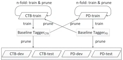
Figure 2:Workflow of offline pruning.

of most likely candidate tags whose accumulative probability is larger thanλ. Then, we only keep the min(r′, r)most likely candidate tags.

We have _|T˜i| = r2 without considering the

ac-cumulated probability thresholdλ. Thus, it requires O(nr4)time complexity to computeE_t|x,S;˜_θ[f(x,t)]

using the Forward-Backward algorithm.

In the following, we propose two ways for real-izing context-aware pruning, i.e., online and offline pruning. Their comparison and analysis are given in the experiment parts.

3.1 Online Pruning

The online pruning approach directly uses the cou-pled model to perform pruning. Given a sentence, we first use a subset of featuresfsep_a(.)and

corre-sponding feature weights trained so far to compute marginal probabilities of first-side tags, and then analogously process the second-side tags based on fsep_b(.). This requires roughly the same time

com-plexity as two baseline models. Then the marginal probabilities are used for pruning.

3.2 Offline Pruning

The offline pruning approach is a little bit more complex, and uses many additional single-side tag-ging models for pruning. Fig. 2 shows the work-flow. Particularly, n-fold jack-knifing is adopted to perform pruning on the same-side training data. Finally, all training/dev/test datasets of CTB and PD are preprocessed in an offline way, so that each word in a sentence has a set of most likely CTB tags (Ta

i )

and another set of most likely PD tags (_Tib).

4 Experiment Settings

data split of CTB5, the training/dev/test datasets contain 16,091/803/1,910sentences respectively. For PD, we use the 46,815 sentences in January 1998 as the training data, the first2,000sentences in February as the development data, and the first 5,000sentences in June as the test data.

Evaluation Metrics. We use the standard token-wise tagging accuracy for POS tagging. For joint WS&POS tagging, besides character-wise tagging accuracy, we also use the standard precision (P), recall (R), and F-score of only words (WS) or POS-tagged words (WS&POS).

Parameter settings. Stochastic gradient descent (SGD) is adopted to train the baseline single-side tagging models, the guide-feature models, and the coupled models.4

For the coupled models, we directly follow the simple corpus-weighting strategy proposed in Li et al. (2015) to balance the contribution of the two datasets. We randomly sample 5,000 CTB-train sentences and5,000PD-train sentences, which are then merged and shuffled for one-iteration training. After each iteration, the coupled model is evaluated on both CTB-dev and PD-dev, providing us two single-side tag accuracies, one on CTB-side tags, and the other on PD-dev tags. Another advantage of using a subset of training data in one iteration is to monitor the training progress in smaller steps. For fair comparison, when building the baseline and guide-feature models, we also randomly sample 5,000 training sentences from the whole training data for one-iteration training, and then report an tagging accuracy on development data. For all mod-els, the training terminates if peak accuracies stop improving within 30 consecutive iterations, and we use the model that performs the best on development data for final evaluation on test data.

5 Experiments on POS Tagging

5.1 Parameter Tuning

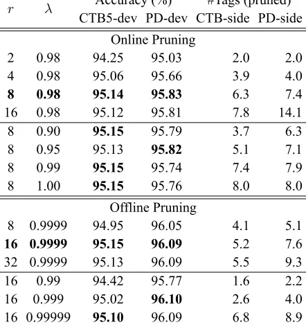
For both online and offline pruning, we need to de-cide the maximum number of single-side tag candi-datesrand the accumulative probability thresholdλ for further truncating the candidates. Table 2 shows

4

We use the implementation of SGD in CRFsuite (http:// www.chokkan.org/software/crfsuite/), and setb = 30

as the batch-size andC= 0.1as the regularization factor.

r λ Accuracy (%) #Tags (pruned)

CTB5-dev PD-dev CTB-side PD-side Online Pruning

2 0.98 94.25 95.03 2.0 2.0

4 0.98 95.06 95.66 3.9 4.0

8 0.98 95.14 95.83 6.3 7.4

16 0.98 95.12 95.81 7.8 14.1

8 0.90 95.15 95.79 3.7 6.3

8 0.95 95.13 95.82 5.1 7.1

8 0.99 95.15 95.74 7.4 7.9

8 1.00 95.15 95.76 8.0 8.0

Offline Pruning

8 0.9999 94.95 96.05 4.1 5.1

16 0.9999 95.15 96.09 5.2 7.6

32 0.9999 95.13 96.09 5.5 9.3

16 0.99 94.42 95.77 1.6 2.2

16 0.999 95.02 96.10 2.6 4.0

16 0.99999 95.10 96.09 6.8 8.9

Table 2:POS tagging performance of online and offline pruning with differentrandλon CTB5 and PD.

the tagging accuracies and the averaged numbers of single-side tags for each token after pruning.

The first major row tunes the two hyper-parameters for online pruning. We first fixλ= 0.98 and increaser from2 to8, leading to consistently improved accuracies on both CTB5-dev and PD-dev. No further improvement is gained withr= 16, indicating that tags below the top-8are mostly very unlikely ones and thus insignificant for computing feature expectations. Then we fix r = 8 and try different λ. We find that λ has little effect on tagging accuracies but influences the numbers of remaining single-side tags. We chooser = 8and λ= 0.98for final evaluation.

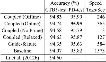
Accuracy (%) Speed CTB5-test PD-test Toks/Sec

Coupled (Offline) 94.83 95.90 246

Coupled (Online) 94.74 95.95 365

Coupled (No Prune) 94.58 95.79 3

Coupled (Relaxed) 94.63 95.87 127

Guide-feature 94.35 95.63 584

Baseline 94.07 95.82 1573

Li et al. (2012b) 94.60 — —

Table 3:POS tagging performance of difference approaches on CTB5 and PD.

5.2 Main Results

Table 3 summarizes the accuracies on the test data and the tagging speed during the test phase. “Cou-pled (No Prune)” refers to the cou“Cou-pled model with complete mapping in Li et al. (2015), which maps each one-side tag to all the-other-side tags. “Coupled (Relaxed)” refers the coupled model with relaxed mapping in Li et al. (2015), which maps a one-side tag to a manually-designed small set of the-other-side tags. Li et al. (2012b) report the state-of-the-art accuracy on this CTB data, with a joint model of Chinese POS tagging and dependency parsing.

It is clear that both online and offline pruning greatly improve the efficiency of the coupled model by about two magnitudes, without the need of a carefully predefined set of tag-to-tag mapping rules.5 Moreover, the coupled model with offline pruning achieves 0.76% accuracy improvement on CTB5-test over the baseline model, and 0.48% over our reimplemented guide-feature approach of Jiang et al. (2009). The gains on PD-test are marginal, possibly due to the large size of PD-train, similar to the results in Li et al. (2015).

6 Experiments on Joint WS&POS Tagging

6.1 Parameter Tuning

Table 4 shows results for tuning r and λ. From the results in the first major row, we can see that in the online pruning method, λseems useless and r becomes the only threshold for pruning unlikely single-side tags. The accuracies are much inferior to

5

Due to the model complexity of “Coupled (No Prune)”, we discard all low-frequency (<3) features in the training data to speed up training. This explains why “Coupled (No Prune)” has slightly lower accuracies than “Coupled (Relaxed)”.

r λ Accuracy (%) #Tags (pruned)

CTB5-dev PD-dev CTB-side PD-side Online Pruning

8 1.00 90.41 89.91 8.0 8.0

16 0.95 90.65 90.22 15.9 16.0

16 0.99 90.77 90.49 16.0 16.0

16 1.00 90.79 90.49 16.0 16.0

Offline Pruning

8 0.995 91.22 91.62 2.6 3.1

16 0.995 91.66 91.85 3.2 4.3

32 0.995 91.67 91.87 3.5 5.6

16 0.95 90.69 91.30 1.6 2.1

16 0.99 91.64 91.92 2.5 3.5

16 0.999 91.62 91.75 5.1 6.4

Table 4:WS&POS tagging performance of online and offline pruning with differentrandλon CTB5 and PD.

those from the offline pruning approach. We believe that the accuracies can be further improved with larger r, which would nevertheless lead to severe inefficiency issue. Based on the results, we choose r= 16andλ= 1.00for final evaluation.

The second major row tries to decider andλfor the offline pruning approach. Under λ = 0.995, increasingrfrom8to16improves accuracies both on CTB5-dev and PD-dev, but further usingr = 32 leads to little gain. Then we fixr = 16 and vary λfrom0.95to0.999. Usingλ = 0.95leaves only 1.6CTB tags and2.1PD tags for each character, but has a large accuracy drop. We chooser = 16and λ = 0.995for offline pruning for final evaluation, which leaves each character with3.2CTB-tags and 4.3PD-tags on average.

6.2 Main Results

Table 5 summarizes the accuracies on the test data and the tagging speed (characters per second) during the test phase. “Coupled (No Prune)” is not tried due to the prohibitive tag set size in joint WS&POS tag-ging, and “Coupled (Relaxed)” is also skipped since it seems impossible to manually design reasonable tag-to-tag mapping rules in this case.

In terms of efficiency, the coupled model with offline pruning is on par with the baseline single-side tagging model.6

6

P/R/F (%) on CTB5-test P/R/F (%) on PD-test Speed Only WS Joint WS&POS Only WS Joint WS&POS Char/Sec Coupled (Offline) 95.65/95.46/95.55 90.68/90.49/90.58 96.39/95.86/96.12 92.70/92.19/92.44 115 Coupled (Online) 95.17/94.71/94.94 89.80/89.37/89.58 95.76/95.45/95.60 91.71/91.41/91.56 26 Guide-feature 95.26/94.89/95.07 89.96/89.61/89.79 95.99/95.33/95.66 91.92/91.30/91.61 27 Baseline 95.00/94.77/94.88 89.60/89.38/89.49 96.56/96.00/96.28 92.74/92.20/92.47 119

Table 5:WS&POS tagging performance of difference approaches on CTB5 and PD.

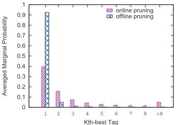
0 0.1 0.2 0.3 0.4 0.5 0.6 0.7 0.8 0.9 1

1 2 3 4 5 6 7 8 >8

A

veraged Marginal Probability

Kth-best Tag

online pruning offline pruning

Figure 3: Probability distribution with online/offline pruning for the task of joint WS&POS.

In terms of F-score, the coupled model with offline pruning achieves 0.67% (WS) and 1.09% (WS&POS) gains on CTB5-test over the baseline model, and 0.48% (WS) and 0.79% (WS&POS) over our reimplemented guide-feature approach of Jiang et al. (2009). Similar to the case of POS tagging, the baseline model is very competitive on PD-test due to the large scale of PD-train.

6.3 Analysis

Online vs. offline pruning. The averaged numbers of single-side tags after pruning in Table 4 and 2), suggest that the online pruning approach works badly in assigning proper marginal probabilities to different tags. Our first guess is that in online prun-ing, the weights of separate features are optimized as a part of the coupled model, and thus producing somewhat flawed probabilities. However, our fur-ther analysis gives a more convincing explanation.

Fig. 3 compares the distribution of averaged probabilities ofkth-best CTB-side tags after online and offline pruning. The statistics are gathered on CTB5-test. Under online pruning, the averaged probability of the best tag is only about0.4, which is surprisingly low and cannot be explained with the

equal to the time of two baseline models.

aforementioned improper optimization issue. Please note that both the online and offline models uses the best choices ofr andλ based on Table 4, and are trained until convergence.

After a few trials of reducing the size of PD-train for training the coupled model, we realize that the underlying reason is that ambiguous labeling makes the probability mass more uniformly distributed, since for a PD-train sentence, the characters only have the gold-standard PD-side tags, and the model basically uses all CTB-side tags as gold-standard answers. Thanks to the CTB-train sentences, the model may be able to choose the correct tag, but inevitably becomes more indecisive at the same time due to the PD-train sentences.

In contrast, the offline pruning approach directly uses two baseline models for pruning, which is a job perfectly suitable for the baseline models. The entropy of the probability distribution for online pruning is about1.524while that for offline pruning is only0.355.

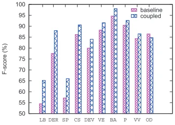
Error distributions. To better understand the gains from the coupled approach, we show the F-score of specific POS tags for both the baseline and coupled models in Fig. 4, in the descending order of absolute F-score improvements. The largest improvement is from words tagged as “LB” (mostly for the word “被”, marking a certain type of passive construction), and the F-score increases by65.22₋ 54.55 = 10.67%. Nearly all POS tags have more or less F-score improvement. Due to the space limit, we only show the tags with more than2.0% improvement. The most noticeable exception is that F-score drops by 84.80 − 86.49 = −1.69% for words tagged as “OD” (ordinal numbers, as opposed to cardinal numbers).

50 55 60 65 70 75 80 85 90 95 100

LB DER SP CSDEV VE BA P VV OD

F-score (%)

baseline coupled

Figure 4:F-score comparison between the baseline and coupled WS&POS tagging models on different CTB POS tags.

F (%) on CTB5X-test Only WS Joint WS&POS Coupled (Offline) 98.01 94.39

Guide-feature 97.96 94.06

Baseline 97.37 93.23

Sun and Wan (2012) — 94.36

Jiang et al. (2009) 98.23 94.03

Table 6: WS&POS tagging performance of difference ap-proaches on CTB5X and PD.

improvement of90.00−16.67 = 73.33% in recall ratio. The reason is that PD-train contains a lot of related words such as “卢森堡” (Luxembourg, place name) and “克 拉 泽 博 格” (Krayzelburg, person name) while CTB5-train has none.

6.4 Comparison with Previous Work

In order to compare with previous work, we also run our models on CTB5X and PD, where CTB5X adopts a different data split of CTB5 and is widely used in previous research on joint WS&POS tagging (Jiang et al., 2009; Sun and Wan, 2012). CTB5X-dev/test only contain 352/348 sentences respectively. Table 6 presents the F scores on CTB5X-test. We can see that the coupled model with offline pruning achieves 0.64% (WS) and 1.16% (WS&POS) F-score improvements over the baseline model, and 0.05% (WS) and 0.33% (WS&POS) over the guide-feature approach.

The original guide-feature method in Jiang et al. (2009) achieves98.23% and94.03% F-score, which is very close to the results of our reimplemented model. The sub-word stacking approach of Sun and Wan (2012) can be understood as a more complex

variant of the basic guide-feature method.7

The results on both the larger CTB5-test (in Ta-ble 5) and CTB5X-test suggest that the coupled approach is more consistent and robust than the guide-feature method. The reason may be two-fold. First, in the coupled approach, the model is able to actively learn the implicit mappings between two sets of annotations, whereas the guide-feature model can only passively learn when to trust the automatically produced tags. Second, the coupled approach can directly learn from both heterogeneous training datasets, thus covering more phenomena of language usage.

7 Related Work

A lot of research has been devoted to design an effec-tive way to exploit non-overlapping heterogeneous labeled data, especially in Chinese language process-ing, where such heterogeneous resources are ubiqui-tous due to historical reasons. Jiang et al. (2009) first propose the guide-feature approach, which is similar to stacked learning (Nivre and McDonald, 2008), for joint WS&POS tagging on CTB and PD. Sun and Wan (2012) further extend the guide-feature method and propose a more complex sub-word stacking ap-proach. Qiu et al. (2013) propose a linear coupled model similar to that of Li et al. (2015). The key difference is that the model of Qiu et al. (2013) only uses separate features, while Li et al. (2015) and this work explore joint features as well.

Li et al. (2012a) apply the guide-feature idea to dependency parsing on CTB and PD. Zhang et al. (2014a) extend a shift-reduce dependency parsing model in order to simultaneously learn and produce two heterogeneous parse trees, which however as-sumes the existence of training data with both-side annotations.

Our context-aware pruning approach is similar to coarse-to-fine pruning in parsing community (Koo and Collins, 2010; Rush and Petrov, 2012), which is a useful technique that allows us to use very complex parsing models without too much efficiency cost. The idea is first to use a simple and basic off-shelf model to prune the search space and only keep highly likely dependency links, and then let the complex

7

model infer in the remaining search space. Weiss and Taskar (2010) propose structured prediction cas-cades: a sequence of increasingly complex models that progressively filter the space of possible outputs, and provide theoretical generalization bounds on a novel convex loss function that balances pruning error with pruning efficiency.

This work is also closely related with multi-task learning, which aims to jointly learn multiple related tasks with the benefit of using interactive features under a share representation (Ben-David and Schuller, 2003; Ando and Zhang, 2005; Parameswaran and Weinberger, 2010). However, as far as we know, multi-task learning usually assumes the existence of data with labels for multiple tasks at the same time, which is unavailable in our scenario, making our problem more particularly difficult.

Our coupled CRF model is similar to a factorial CRF (Sutton et al., 2004), in the sense that the bundled tags can be factorized into two connected latent variables. Initially, factorial CRFs are de-signed to jointly model two related (and typically hierarchical) sequential labeling tasks, such as POS tagging and chunking. In this work, our coupled CRF model jointly handles two same tasks with different annotation schemes. Moreover, this work provides a natural way to learn from incomplete annotations where one sentence only contains one-side labels.

Learning with ambiguous labeling is previously explored for classification (Jin and Ghahramani, 2002), sequence labeling (Dredze et al., 2009), parsing (Riezler et al., 2002; Täckström et al., 2013). Recently, researchers propose to derive natural annotations from web data to supervise Chinese word segmentation models in the form of ambiguous labeling (Jiang et al., 2013; Liu et al., 2014; Yang and Vozila, 2014).

8 Conclusion

This paper proposes a context-aware pruning ap-proach for the coupled sequence labeling model of Li et al. (2015). The basic idea is to more accurately constrain the bundled tag space of a token according to its contexts in the sentence, instead of using heuristic context-free tag-to-tag mapping rules in the original work. We propose and compare two

different ways of realizing pruning, i.e., online and offline pruning. In summary, extensive experiments leads to the following findings.

(1) Offline pruning works well on both POS tag-ging and joint WS&POS tagtag-ging, whereas on-line pruning only works well on POS tagging but fails on joint WS&POS tagging due to the much larger tag set. Further analysis shows that the reason is that under online pruning, ambiguous labeling during training makes the probabilities of single-side tags more evenly distributed.

(2) In terms of tagging accuracy and F-score, the coupled approach with offline pruning outper-forms the baseline single-side tagging model by large margin, and is also consistently better than the mainstream guide-feature method on both POS tagging and joint WS&POS tagging.

Acknowledgments

The authors would like to thank the anonymous reviewers for the helpful comments. We are very grateful to Meishan Zhang for inspiring us to use online pruning to improve the efficiency of the cou-pled approach. We also thank Wenliang Chen for the helpful discussions. This work was supported by National Natural Science Foundation of China (Grant No. 61525205, 61502325, 61432013).

References

Rie Kubota Ando and Tong Zhang. 2005. A framework for learning predictive structures from multiple tasks and unlabeled data. Journal of Machine Learn Research, 6:1817–1853.

Shai Ben-David and Reba Schuller. 2003. Exploiting task relatedness for multiple task learning. InCOLT. Mark Dredze, Partha Pratim Talukdar, and Koby

Cram-mer. 2009. Sequence learning from data with multiple labels. InECML/PKDD Workshop on Learning from Multi-Label Data.

Wenbin Jiang, Liang Huang, and Qun Liu. 2009. Au-tomatic adaptation of annotation standards: Chinese word segmentation and POS tagging – a case study. InProceedings of ACL, pages 522–530.

Wenbin Jiang, Meng Sun, Yajuan Lü, Yating Yang, and Qun Liu. 2013. Discriminative learning with natural annotations: Word segmentation as a case study. In

Rong Jin and Zoubin Ghahramani. 2002. Learning with multiple labels. InProceedings of NIPS.

Terry Koo and Michael Collins. 2010. Efficient third-order dependency parsers. InACL, pages 1–11. John Lafferty, Andrew McCallum, and Fernando Pereira.

2001. Conditional random fields: Probabilistic models for segmenting and labeling sequence data. In

Proceedings of ICML 2001, pages 282–289.

Zhenghua Li, Wanxiang Che, and Ting Liu. 2012a. Exploiting multiple treebanks for parsing with qua-sisynchronous grammar. InACL, pages 675–684. Zhenghua Li, Min Zhang, Wanxiang Che, and Ting

Liu. 2012b. A separately passive-aggressive training algorithm for joint POS tagging and dependency parsing. InCOLING, pages 1681–1698.

Zhenghua Li, Jiayuan Chao, Min Zhang, and Wenliang Chen. 2015. Coupled sequence labeling on heterogeneous annotations: POS tagging as a case study. InProceedings of ACL, pages 1783–1792. Yijia Liu, Yue Zhang, Wanxiang Che, Ting Liu, and

Fan Wu. 2014. Domain adaptation for CRF-based Chinese word segmentation using free annotations. In

Proceedings of EMNLP, pages 864–874.

Joakim Nivre and Ryan McDonald. 2008. Integrating graph-based and transition-based dependency parsers. InProceedings of ACL, pages 950–958.

S. Parameswaran and K.Q. Weinberger. 2010. Large margin multi-task metric learning. In J. Lafferty, C. K. I. Williams, J. Shawe-Taylor, R.S. Zemel, and A. Culotta, editors, Advances in Neural Information Processing Systems 23, pages 1867–1875.

Xipeng Qiu, Jiayi Zhao, and Xuanjing Huang. 2013. Joint Chinese word segmentation and POS tagging on heterogeneous annotated corpora with multiple task learning. InProceedings of EMNLP, pages 658–668. Stefan Riezler, Tracy H. King, Ronald M. Kaplan,

Richard Crouch, John T. III Maxwell, and Mark Johnson. 2002. Parsing the wall street journal using a lexical-functional grammar and discriminative estimation techniques. InProceedings of ACL, pages 271–278.

Alexander Rush and Slav Petrov. 2012. Vine pruning for efficient multi-pass dependency parsing. In

Proceedings of NAACL-2012, pages 498–507. Weiwei Sun and Xiaojun Wan. 2012. Reducing

approximation and estimation errors for Chinese lexical processing with heterogeneous annotations. In

Proceedings of ACL, pages 232–241.

Charles Sutton, Khashayar Rohanimanesh, and Andrew McCallum. 2004. Dynamic conditional random fields: Factorized probabilistic models for labeling and segmenting sequence data. In International Conference on Machine Learning (ICML).

Oscar Täckström, Ryan McDonald, and Joakim Nivre. 2013. Target language adaptation of discriminative transfer parsers. In Proceedings of NAACL, pages 1061–1071.

David Weiss and Ben Taskar. 2010. Structured prediction cascades. InProceedings of International Conference on Artificial Intelligence and Statistics (AISTATS). Fei Xia. 2000. The part-of-speech tagging guidelines for

the penn Chinese treebank 3.0. InTechnical Report, Linguistic Data Consortium.

Nianwen Xue, Fei Xia, Fu-Dong Chiou, and Martha Palmer. 2005. The Penn Chinese Treebank: Phrase structure annotation of a large corpus. In Natural Language Engineering, volume 11, pages 207–238. Fan Yang and Paul Vozila. 2014. Semi-supervised

Chinese word segmentation using partial-label learn-ing with conditional random fields. InProceedings of EMNLP, pages 90–98.

Shiwen Yu, Huiming Duan, Xuefeng Zhu, Bin Swen, and Baobao Chang. 2003. Specification for corpus processing at Peking University: Word segmentation, POS tagging and phonetic notation (In Chinese). Jour-nal of Chinese Language and Computing, 13(2):121– 158.

Yue Zhang and Stephen Clark. 2008. Joint word segmen-tation and POS tagging using a single perceptron. In

Proceedings of ACL-08: HLT, pages 888–896. Meishan Zhang, Wanxiang Che, Yanqiu Shao, and Ting

Liu. 2014a. Jointly or separately: Which is better for parsing heterogeneous dependencies? InProceedings of COLING, pages 530–540.