Deterministic Deployment of Wireless Sensor Networks

Deterministic Deployment of Wireless Sensor

Networks

∗

M. Brazil

_{C. J. Ras}

_{D. A. Thomas}

Abstract—We propose a new heuristic for deter-ministic deployment of wireless sensor networks when

1-connectivity and minimum cost are the two com-peting objectives. Given a set of data sources and a base station, our aim is to introduce the minimum number of relays to the network so that every sen-sor is connected to the base station via some multi-hop path. We assume that the data sources and base station lie in a plane, and that every sensor and re-lay has the same fixed communication radius. Our heuristic is based on the GEOSTEINER algorithms for the Steiner minimal tree problem, and proves to be much more accurate than the current best heuris-tics for the 1-connected deployment problem, espe-cially in the case of sparse data source distributions.

Keywords: wireless sensor networks, connectivity, de-terministic deployment, Steiner trees

1

Introduction

A wireless sensor network (WSN) consists of small sens-ing devices that can be readily deployed in diverse envi-ronments to form a distributed wireless network for col-lecting information in a robust and autonomous manner. Although early research was mainly motivated by poten-tial military uses, there are now many other important applications such as fault detection, environmental habi-tat monitoring, irrigation and terrain monitoring (see, eg, [1], [9]). As an example of the latter, many lives have re-cently been lost in Australia due to bush fires. An early warning system is critical in preventing small fires from becoming disastrous infernos. Deploying smart sensors in strategically selected areas can lead to early detection and an increased likelihood of success in fire extinguishing efforts. There are also many medical applications includ-ing monitors and implantable devices as well as smart sensors for pollution control and climate control in large buildings.

A sensor network can be deployed in two ways: with de-terministic placement, where a particular quality of ser-vice can be guaranteed; or with random placement, where

∗_{This research was supported by an ARC Discovery Grant.} †_{Department of Electrical and Electronic Engineering,}

The University of Melbourne, Victoria 3010, Australia; brazil@unimelb.edu.au.

‡_{Department of Mechanical Engineering, University of}

Mel-bourne; doreen.thomas@unimelb.edu.au.

sensors are scattered possibly from an aircraft. Although many consider random placement to be the ultimate long term goal, it is currently infeasible in most situations as the individual sensors are generally too expensive for this level of redundancy (in many cases costing thousands of dollars each), and, under current technologies, often need to be carefully set up by hand. Note also that the de-terministic case, where we can control placement of the nodes, provides a lower bound on the number of nodes needed to cover the area and hence is useful for the ran-dom model where the density of the sensors is a significant factor in performance. Randomly deployed WSNs may also be augmented (for any of a number of reasons) by deterministically deploying additional sensors or relays. For these reasons this paper will focus on deterministic deployment only.

The topic of this paper is the most fundamental objec-tive of deployment of wireless sensor networks, namely 1-connectivity. Although it is possible to interconnect a WSN in many ways, we define 1-connectivity as the exis-tence of at least one multi-hop path between every sensor in the network and the base station. This is the most ba-sic requirement for the functioning of the network and can primarily be achieved in two ways: through power level adjustment (we will not consider this option here, but see [11] as a starting point for further study), or by deploying extra sensors or relays (see for instance [4]). The competing objective when deploying relays for con-nectivity is cost, which is predominantly determined by the number of added relays. Consequently our aim will be to deploy the minimum number of relays needed in or-der to ensure connectivity. We make the assumption that every sensor and relay in the network has the same com-munication radius, and by scaling we may assume that this radius is 1 unit.

in the literature, and an optimal solution is called a min-imum Steiner point tree.

The MSPT problem was first described by Sarrafzadeh and Wong in [12], where they showed that it is NP-complete. Consequently a fair amount of research has been directed towards finding good heuristics. In [8] the minimum spanning tree (MST) heuristic was introduced (note that there they refer to the MSPT problem as the

Steiner tree problem with minimum number of Steiner points and bounded edge length, or STP-MSPBEL). This heuristic simply subdivides all edges of an MST that are longer than one unit, resulting in an approximate MSPT solution within polynomial time. Mandoiu and Zelikovsky [10] prove that, in any metric space, the per-formance ratio of the MST heuristic is always one less than the maximum possible degree of a minimum-degree MST spanning points from the space. This gives an ap-proximation ratio of four in the Euclidean plane and three in the rectilinear plane. Chen et al. [3] provide an im-proved approximation scheme, partly based on the MST heuristic, which has a performance ratio of three in the Euclidean plane.

The MSPT problem may be seen as a variant of the clas-sical Steiner tree problem, which asks for a shortest tree interconnecting a set of nodes where any number of ad-ditional nodes may be introduced. An optimal solution to this problem is called a Steiner minimal tree (SMT). As the minimum distance between the given nodes tends to infinity, an SMT with subdivided edges becomes an optimal solution to the MSPT problem. This leads us to the question: would the SMT approximation for the MSPT problem be a practical and accurate heuristic? Certainly we do not have effective algorithms for calcu-lating SMT’s for very large sets of nodes, in fact the prob-lem is NP-hard. However, Warme, Winter, and Zachari-asen ([13],[14]) have developed practical, fast and optimal SMT algorithms for up to thousands of points, namely the GEOSTEINER algorithms.

In this paper we define and analyze theSMT heuristicfor MSPTs. We provide a small linear upper bound in terms of the number of original data sources (sensors) for the performance difference of the SMT heuristic, and show that this bound is best possible in the Euclidean plane.

2

Preliminaries

Consider a set N ⊆ R2_{. TheSteiner tree problem asks}

for a shortest tree interconnectingN, where extra nodes

W ⊂ R2 _{are introduced if they reduce the total length.}

Introducing degree one or degree two nodes will not re-duce total length, henceforth for the Steiner tree problem we assume all added nodes are of degree at least three. The nodes inN are calledterminal points and the nodes inW are calledSteiner points.

In our discussions we distinguish between the concept of a free node and an embedded node. In other words any tree may be considered as a topological graph structure only, or as an embedded network. Embedded nodes are denoted by bold letters (as is common when representing vectors).

Two standard techniques for shortening an embedded tree are splitting and Steiner point displacements. To

split a nodev one disconnects two or more of the edges atv and connects them instead to a new Steiner point, connected tov by an extra edge. To displace a Steiner point one simply embeds it at any new point in the plane without changing the topology of the tree. If no short-ening of a tree is possible when splitting or Steiner point displacements are allowed, then the tree is called aSteiner tree. Note that an SMT is always a Steiner tree. A full Steiner tree is a Steiner tree where every terminal is of degree one and every Steiner point is of degree three. A full Steiner tree has exactly|N| −2 Steiner points and 2|N| −3 edges. A cherry of a full Steiner tree is the subtree induced by two terminals and their mutually ad-jacent Steiner point. Every full Steiner tree has at least two cherries. We refer the reader to [6] and [7] for more background on Steiner trees.

Given two pointsx,y∈R2_{, we denote the edgeebetween}

them by e = xy, and we use the standard notation |e| to denote x−y. Any Steiner tree can be viewed as a candidate MSPT if we simply subdivide, or bead, edges that are longer than one unit. Formally, beading is the process whereby for every edgee,|e|−1 equally spaced degree-two nodes lying oneare included (along with the elements of W) in the set U of extra MSPT nodes. In general, any tree can be viewed as an MSPT candidate if we partition its nodes into a set N of terminals and a set W of Steiner points of degree at least three, and then bead any edges that are too long. Consequently, when constructing an MSPT on a given set N, we are mainly concerned with finding the elements of W, i.e. the elements ofU that have degree at least three; clearly degree one nodes will not occur inUand degree two nodes in U only arise from beading. Henceforth, degree two nodes inU will not be considered as part of the topology of the MSPT. All nodes inU will be referred to asbeads

and, specifically, the nodes in W will be called Steiner beads. The procedure of constructing an SMT in order to approximate an MSPT will be referred to as theSMT heuristic.

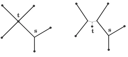
heretis a degree-four terminal,sis a Steiner point, and after splittingtwe have three zero-length edges (depicted by broken lines).

t

t s

s

Figure 1: Conversion to a full Steiner tree

Let the edge-set of T∗ be E(T∗) = {e₁, ..., e_m}, where

m = 2n−3. Then the bead count ofT is beads(T) =

|U|=n−2 +m_i=1(|ei| −1) = 1−n+m_i=1|ei|. In

other words, by considering _T∗ rather than _T we get a formula for beads(T) that does not depend on the number of Steiner beads of T; this formula works because every time a node is split (creating a new Steiner bead) we introduce a zero-length edge which in effect cancels the count of this Steiner bead. We can now reformulate the MSPT problem as follows: letN be a subset ofR2_{. Find}

aW ⊂R2_{and a treeT interconnectingN∪W such that}

every node inW is of degree at least three and beads(T) is a minimum over all trees interconnectingN.

3

The Upper Bound

In this section we provide an upper bound for the perfor-mance difference of the SMT heuristic. Let N be a set of n terminals in the Euclidean plane. We use Topt to

denote an MSPT onN andTS to denote an SMT onN.

We need the following lemma before we prove our main result:

Lemma 1 Ifi, kare real numbers theni+k−i=k

ork−1(equivalentlykork+1), withi+k−i=

kif kis an integer.

Proof. Suppose that i= i+εi and k =k+εk

where 0≤εi, εk<1. Theni+k=i+k−εi+εk,

from which the result follows.

Suppose that E(T_opt∗ ) = {e1, ..., em} and E(TS∗) = {a1, ..., am}. Then

m

i=1|ai| ≤ m

i=1|ei|

sinceT_S is a shortest total length tree connectingN. We can therefore parti-tion the set {1, ..., m} as follows: let{1, ..., m}= I∪D such that|ei|=|ai|+pi fori∈I and|ei|=|ai| −pi for i ∈D. Here each p_i is a non-negative real number and the cardinality ofD, but notI, may be zero. We further partitionIintoIZandIZ (whereIZ may be empty) such

thati∈IZ if and only if|ai| is an integer. We similarly

partitionDintoDZ and DZ. Note that i∈Ipi≥

i∈Dpi

-an inequality that is central to the next proof.

Proposition 2 beads(TS)−beads(Topt)≤ 2n−4−j,

where j is the number of integer-length edges inE(T_S∗).

Proof.

beads(TS)−beads(Topt)

=

1−n+

m

i=1

|ai|

−

1−n+

m

i=1

|ei|

=

m

i=1

|ai| − m

i=1

|ei|

=

i∈D

{|ai| − |ai| −pi} −

i∈I

{|ai|+pi − |ai|}.

Therefore, if somepi∈/Zfori∈I then:

beads(TS)−beads(Topt)

≤

i∈DZ

pi+

i∈D

Z

(p_i+ 1)−

i∈IZ

pi

−

i∈I

Z

(pi −1)

=|D_Z|+|I_Z|+

i∈D pi −

i∈I pi

≤m−j+

i∈I pi−

i∈I pi < m−j

= 2n−3−j.

Similarly, ifp_i∈Zfor alli∈I then: beads(TS)−beads(Topt)

≤

i∈DZ

pi+

i∈D

Z

(p_i+ 1)−

i∈I pi

≤m− |I| −j < m−j.

Corollary 3 beads(T_S)−beads(T_opt)≤2n−c−3where

c is the number of full components of TS.

Proof. Note that every terminalxof degree deg(x) is split deg(x)−1 times to produceT_S∗, i.e. each terminal

x produces deg(x)−1 zero-length edges after all splits. Clearly alsoc=

Corollary 4 IfTShas at most one edge with non-integer

length thenbeads(TS) = beads(Topt).

Du et al. in [3] and [5] provide an approximation for the MSPT problem that gives a performance ratio with upper bound of three in the Euclidean plane. Their algo-rithm is based on the MST heuristic and therefore runs in polynomial time. If we rewrite our performance differ-ence to get the bounded ratio beads(TS)

beads(Topt) ≤1 +beads(2n−T4opt)

we see that the performance ratio of the SMT heuristic has a smaller upper bound than the heuristic of Du et al. when beads(Topt) > n−2. Since beads(Topt) increases

as the minimum distance between any pair of terminals increases, we arrive at the intuitive fact that the per-formance of the SMT heuristic improves as the terminal configuration becomes more sparse. During this limiting process the upper bound of the ratio beads(TM)

beads(TS), whereTM

is an MST, tends towards the well-known Steiner ratio. This gives a limiting upper bound of beads(TM)

beads(TS) ≤

√

3 2 in

the Euclidean plane, which serves as a comparison be-tween the performances of the SMT heuristic and the standard MST heuristic.

We mention once again that the SMT heuristic does not run in polynomial time. However, fornup to a few thou-sand nodes the GEOSTEINER algorithms will produce solutions in reasonable running time. This makes the SMT heuristic a tool worthy of consideration for applica-tions where optimization is required during an initializa-tion process (such as deployment) and the cost benefit of a more accurate algorithm justifies a possible time delay.

4

Sharpness of the Upper Bound

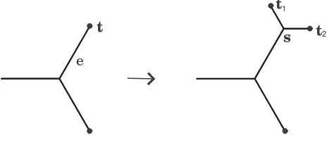
The aim of this section is to show that the performance difference from Proposition 2 is best possible. We begin with a few definitions and preliminary results. Due to minimality of total length, any two adjacent edges of a Euclidean Steiner tree meet at an angle of at least 120◦. This implies that the degree of any terminal is no more than 3, and the degree of any Steiner point is exactly 3. Let T be a full Steiner tree on a set of embedded ter-minals. To sprout new terminals from a given terminal

t of T, with incident edgee one replacest by a Steiner pointsand embeds two new terminalst₁,t₂adjacent tos

such that the two new edgesst1 andst2each form 120◦

angles with e and with each other - see Figure 2. We denote by L(T) the total Euclidean edge length ofT. If

N is a set of embedded terminals thenTS will denote a

Euclidean SMT on N and T_opt will denote a Euclidean MSPT onN. As usual we letn=|N|. The next proposi-tion shows that we can use sprouting to create full SMTs with any given topology. It is a fundamental result and is almost certainly known, but does not appear to have been explicitly written up in the literature before now.

t

t

t

s

e

Figure 2: Sprouting new terminals

Proposition 5 Given any full Steiner topology, there ex-ists a set of embedded terminals N such that the SMT for N has the given topology and is unique. Further-more, such trees can be explicitly constructed for any given topology.

Proof. LetG_nbe a full Steiner topology onn nals. We will show how a suitable set of embedded termi-nalsN_ncan be constructed by induction onn, where the inductive step involves sprouting new terminals. Note that the construction is trivial if n= 1,2 or 3. The in-ductive claim is as follows.

Claim: For any full Steiner topology,Gi, oniterminals

(withi≥4), there exists a set of embedded terminalsNi

and a real numberfi>0 such that

1. the SMT,Ti, forNi has topologyGi, and

2. ifT_i is a Steiner tree forNi such that the topology

ofT_i is notG_i, thenL(T_i)−L(T_i)≥f_i.

For the base case of the claim (i = 4), choose N4 to

be the four points with coordinates (±3/2,±√3/2). It is easily checked that the SMT T₄ for N₄ has Steiner points (±1/2,0) and length 5 (see Figure 3). The short-est Steiner tree T₄ with a different topology is full with Steiner points (0,±(√3/2−1/(3))) and lengthL(T₄) = 3√3. So we can choosef4= 3

√

3−5 > 0. Up to rela-belling of the terminals, there is only one full topology for i= 4, so this completes the base case.

We now establish the inductive step for (i= n), where we assume that the claim holds for i= n−1. Given a full Steiner topology Gn (n >4), this topology contains

at least one cherry. Replacing such a cherry by a single terminal t∗ gives a full Steiner topology G_n−1 on n− 1 terminals. By the inductive assumption there exists an embedded terminal set N_n−1with unique SMTT_n−1 which has topology Gn−1 and a corresponding constant

fn−1>0. Lettbe the embedded terminal corresponding

1

1

1

1

1

Figure 3: Base case

We sprout new terminals t_n and t_n−1 from t, with t

replaced by a Steiner points, such that|stn−1|=|stn|= fn−1/4. Let this new tree beTnwith embedded terminal

setNn. By construction,Tnhas the correct topologyGn.

LetT_n be any Steiner tree (but not necessarily an SMT) onNnwith topologynot Gn. Suppose we collapsetnand tn−1 into the point s, and consider the resulting

topol-ogy G of this network. If G = Gn−1, then Tn also has

the same topology as T_n, which by convexity and the fact that T_n is a Steiner tree implies thatT_n = Tn (see

Theorem 1.3 of [7]); this is a contradiction and hence

G =Gn−1. It follows from this that, if we consider the

networkT_n∪ {st_n}(which interconnectsN_n−1), we have

L(T_n) +|stn| ≥L(Tn−1) +fn−1. This implies that

L(T_n) ≥ L(T_n−1) + (f_n−1− |st_n|)

> L(T_n−1) + 3|st_n|=L(T_n) +|st_n|.

Hence, we can choose fn=fn−1/4< L(Tn)−L(Tn).

The claim (and lemma) now follow. Furthermore, the iterative algorithm for constructing a suitable set of em-bedded terminals for any required Steiner topology is con-structive withf_i= (3√3−5)/4i−4 _{for eachi≥4.}

The next proposition shows that the upper bound from Proposition 2 is sharp.

Proposition 6 Let Gn be a full Steiner topology on n terminals. There exists an embedded set of termi-nals N in the Euclidean plane such that beads(TS) =

beads(T_opt) + 2n−4and T_S has topologyG_n.

Proof. We construct an SMT TS with topology Gn by repeatedly sprouting terminals, starting from a

full Steiner tree on three terminals called the base. By the previous proposition any full Steiner topology can be produced in this way. By making the edges of the base large enough, it is clear that we can construct TS such

that every edge-length has the forma_i±ε_i, wherea_i is an integer of order at least two andεihas any predefined

value between zero and one. TSis then converted into an

MSPT by a sequence of displacements (which we describe

below) of the Steiner points, where displacements do not change the original topology Gn.

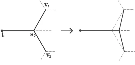
In TS, let s0 be a Steiner point adjacent to a terminalt

and two other nodesv1,v2where edge-lengths are

prese-lected as follows: |ts0|=a1−ε,|s0v1|=|s0v2|=b1+ε1

for large integers a₁, b₁ and 0 < ε, ε₁ < 1. In the first step (Figure 4) we displace s0 along the line through t

and s₀ and in the direction of the vector −→ts₀. We dis-place until |ts0|=a1−ε and|s0v1|=|s0v2|=b1−ε1

for some 0 < ε, ε₁ < 1. Clearly this is possible as long as we preselect ε1 to be small enough compared toε.

s

t

v

v

Figure 4: First step of the displacement sequence

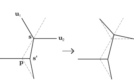
We now displace all other Steiner points in a depth-first or breadth-first order rooted at t. Suppose that in the process we have reached the Steiner pointswith parents

and childrenu1,u2. We displacesalong the line through sand the pointpand in the direction−ps→, wherepis the position s had before its displacement; see Figure 5. If

|ss| = a−ε₁ then we preselect |su₁| = |su₂| = b+ε₂ for 0 < ε2 < 1. We select ε2 small enough so that the

displacement ofsproduces the lengths|ss|=a−ε₁and

|su₁| = |su₂| = b−ε₂, for some 0 < ε₁, ε₂ < 1. We continue this process until we have displaced all Steiner points. Call the resultant tree T. Note that the edges ofTS were preselected so that one edge has lengtha1−

ε and every other edge e_i has length b_i+ε_i. After all displacements the first edge has length a1−ε and every

other ei has length bi−εi. Clearly then beads(TS) =

beads(_T) + 2_n−4 and_T is an MSPT.

5

Conclusions and Future Work

p

s

s'

u

u

Figure 5: General step of the displacement sequence

Extensive simulations have been performed for the GEOSTEINER algorithm (see for instance [13]), so we will not repeat them here. These simulations show that one can calculate SMTs efficiently for up to about two thousand terminals. We therefore believe that the SMT heuristic will become a valuable tool for WSN deploy-ment, especially in applications such as habitat and ter-rain monitoring where, indeed, data-sources distributions are often sparse and seldom contain more than a couple of thousand individual sources. Of course, any deter-ministically deployed WSN is unlikely to consist of an extremely large number of sensors, which means that the SMT heuristic is generally suitable for most of these sce-narios.

Computational and theoretical results have led us to be-lieve that it is possible to improve the performance of the SMT heuristic even more by small displacements of the Steiner points. One of the ways we wish to explore this possibility in the future is through extensive simulations.

Acknowledgement. We wish to thank Jamie Evans for providing many fruitful ideas during the development of this paper.

References

[1] T. Arampatzis, L. Lygeros, J. S. Manesis, “A Sur-vey of Applications of Wireless Sensors and Wireless Sensor networks,” Proc. 13th Mediterranean Conf. on Control and Automation(2005), pp. 719–724. [2] J.–H. Chang, R.–H. Jan, “An Efficient Relay Sensors

Placing Algorithm for Connectivity in Wireless Sen-sor Networks,”Lecture Notes in Computer Science -Embedded and Ubiquitous Computing, 4096 (2006), pp. 874–883.

[3] D. Chen, D.–Z. Du, X.–D. Hu, G.–H. Lin, L. Wang, G. Xue, Approximations for Steiner trees with min-imum number of Steiner points, Theoretical Com-puter Science, 262 (2001) pp. 83–99.

[4] X. Cheng, D.–Z. Du, L. Wang, B. Xu, Relay sen-sor placement in wireless sensen-sor networks, Wireless Networks, 14 (2008), pp. 347–355.

[5] D.–Z. Du, X. Hu, Steiner tree problems in computer communication networks, World Scientific Publish-ing Company, 2008.

[6] E. N. Gilbert, H. O. Pollak, Steiner minimal trees,

SIAM J. Appl. Math., 16 (1968), pp. 1–29.

[7] F. K. Hwang, D. S. Richards, P. Winter, The Steiner Tree Problem, Annals of Discrete Mathematics 53, Elsevier Science Publishers B.V., Amsterdam, 1992.

[8] G.–H. Lin, G.L. Xue, Steiner tree problem with min-imum number of Steiner points and bounded edge– length, Inform. Process. Lett., 69 (1999), pp. 53-57. [9] A. Mainwaring, J. Polastre, R. Szewczyk, D. Culler and J. Anderson, “Wireless Sensor Networks for Habitat Monitoring,” First ACM International Workshop on Wireless Sensor Networks and Appli-cations (WSNA)(2002), pp. 88–97.

[10] I. I. Mandoiu, A. Z. Zelikovsky, A note on the MST heuristic for bounded edge–length Steiner trees with minimum number of Steiner points,Inform. Process. Lett., 75 (2000), pp. 165-167.

[11] M. Naserian, K. Tepe, T. Mohammed, “On the Con-nectivity of Nodes in Wireless Ad Hoc and Sensor Networks,” Canadian Conference on Electrical and Computer Engineering(2005), pp. 2073–2075. [12] M. Sarrafzadeh, C.K. Wong, Bottleneck Steiner trees

in the plane, IEEE Trans. Comput., 41 (1992), pp. 370–374.

[13] D. M. Warme, P. Winter, M. Zachariasen. Exact Al-gorithms for Plane Steiner Tree Problems: A Com-putational Study. In D.–Z. Du, J. M. Smith, J. H. Rubinstein, editors, Advances in Steiner Trees, pp. 81-116, Kluwer Academic Publishers, Boston, 2000.