Ratio Rules Mining in Concept Drifting Data Streams

Ratio Rules Mining in Concept Drifting Data Streams

Wei Fan

∗

Toyohide Watanabe

†

Koichi Asakura

‡

Abstract—Ratio rules mining in data streams is a challenging problem in terms of two issues: con-cept drifting and continuous large amount of data. In this paper, we propose to estimate distribution of each data stream as time progresses, and to detect partially coagulated intervals in the distribution of each data stream as emerging trends. Then we mine ratio rules from subsequences data at these emerg-ing trends. Traditional techniques cannot be applied to process continuous large amount of data in data streams because of time and space constraints. In this paper, we propose an incremental Principle Compo-nent Analysis method, as well as a multiple regres-sion measurement to mine ratio rules incrementally and adaptively. Methods are proposed to detect the change of data trends and to mine ratio rules in a single on-line scan of the data streams. Our exten-sive experiments on synthetic and real datasets verify efficiency and effectiveness of our proposed methods.

Keywords: Ratio rules mining, data streams, emerg-ing trends of data, incremental Principal Component Analysis, multiple regression measurement

1

Introduction

Different from association rule mining [1], ratio rule min-ing is proposed to capture quantitative association knowl-edge [2, 3, 4, 5]. A classical example is {bread : milk :

butter}= 1 : 2 : 1. This example attempts to character-ize purchasing activity:“if a customer spends 1 amount on bread, then s/he is likely to spend 2 amounts on milk and 1 amount on butter“. Although techniques for min-ing ratio rules in static database have been proved to be effective, how to mine ratio rule in concept drifting data streams is still a challenging problem.

Data streams environment imposes additional constraints for the mining procedure: presence of concept drifting and continuous large amount of data. Take the example of market basket data streams. If purchasing activities show an increasing trend in the number of customers with a certain combination of demographic characteristics in a short period, then the manager may be interested in

∗_{Nagoya University, Graduate School of Information Science,}

Nagoya, 464-8603, Japan. Email:

[email protected]

†_{Nagoya University, Graduate School of Information Science,}

Nagoya, 464-8603, Japan. Email: [email protected]

‡_{Daido University, School of Informatics, Nagoya, 457-8530,}

Japan. Email: [email protected]

mining ratio rules at this emerging trend in order to de-scribe the purchasing behavior of this group. On the other hand, traditional techniques cannot be applied to process continuous large amount of data in data streams because of time and space constraints.

In order to address the issues, we propose an approach to mine ratio rules at emerging trends of data streams incre-mentally and adaptively. In order to detect the emerging trends of data streams, we estimate the distribution of the continuous data in each data stream, and detect par-tially coagulated intervals in the distribution of data as the emerging trends. The emerging trends of all data streams can be detected synchronously in a single on-line scan of data. Then we mine ratio rules from subsequences data at these emerging trends. Here, in addition to adopt an automated incremental Principal Component Analysis method for generating ratio rules, we also propose a gen-eralized multiple regression measurement which attempts to assess how good the generated ratio rules are at each new arrival data point.

This paper is organized as follows. In Section 2, we dis-cuss related work for mining ratio rules. Section 3 gives a formal definition of ratio rules. In Section 4 and Section 5, we elaborate our proposed approaches for tackling two issues of our ratio rules mining problem. In Section 6, we present empirical results of synthetic and real data. Finally, Section 7 concludes the paper.

2

Related Work

In [2], ratio rules are defined as eigenvectors of a database (matrix) whose eigenvalues are the largest. This model has the advantage to estimate missing values in the database. While, it also limits the application of ra-tio rules mining in data streams: first, the technique of eigen-analysis cannot be applied to process large volume of continuous data because of time and space constraints. Second, because the mining results in [2] are very easy to fall victim to noise, it is difficult to mine “local” ratio rules which are derived from subsets of data. Third, it is hard to quantify a ratio rule, such as how well does a ratio rule fit to the data streams.

mine ratio patterns from the multidimensional database. However, for data streams, the traditional algorithms for counting support in static database are not efficient.

The authors of [5] proposed an integrated method to mine ratio rules from distributed and changing data source. Similar to our adopted method for mining ratio rules incrementally, a novel robust and adaptive one-pass al-gorithm (RARR) is proposed. However, in our proposed approach, we declare the ratio rules at emerging trends of data, and give a measurement to evaluate the goodness-of-fit of the ratio rules. In our experimental results, we compare the quality of our algorithm with that of RARR.

3

Problem Definition

Let A = {a1, a2,· · ·, am} be a set of attributes which are also the names of the multiple data streams. Anm -dimensional data pointTiarrives ati-th time point, and the value of attributeaj is represented byv(aj).

We define a ratio rule P is a set of emerging trend in terms of a reference attribute and a ratio among at-tributes which is generated from data points at the emerg-ing trend. For example,

P={(a1:a2:a3) = (1 : 2 : 3) ata1∈[1,3]}

represents that at the emerging trend of attribute a1 as

[1,3], ratio relationships among attributes a1, a2 and a3

are v(a2)/v(a1) = 2 : 1, and v(a3)/v(a1) = 3 : 1. Here,

the attributea1is called reference attribute whose values

appear an emerging trend. We omit the attributes whose values are very close to 0, and attributes are ordered in alphabetic order.

In the following sections, we will elaborate the methods to detect emerging trends and to mine ratio rules at the emerging trends incrementally and adaptively.

4

Detection of Emerging Trends

Based on the technique proposed in [6] for diagnosing evolution of data streams, we detect partially coagulated intervals in the distribution of data as emerging trend intervals.

4.1

Change Diagnosis of Data Streams

When a data stream shows high level of evolution, it is expected that the relative data concentrations at various spatial locations may change over time. The work of [6] is able to capture such changes using the concept of velocity density which measures the rate of change of data con-centration at a given spatial location over a user-defined time horizonht.

Let T be the current instant and S be the set of data points which have arrived in the time window (T−ht, T).

(1)

min max

(2)

min max

(3)

min max

(4)

min max

(7)

min max

(5)

min max

(6)

min max

(8)

min max

(1)

min max

(2)

min max

(3)

min max

(4)

min max

(7)

min max

(5)

min max

(6)

min max

(8)

min max

Figure 1: The possible relative positions of coagulation intervals att and (t−1), and dissolution interval att.

We intend to estimate the rate of increase in density at spatial locationX and timeT by using two estimations:

forward time slice density estimation F(hs,ht)(X, T) and

reverse time slice density estimation R(hs,ht)(X, T). In-tuitively,F(hs,ht)(X, T) measures the density function for all spatial locations at a given time tbased on the set of data points which have arrived in the past time window (T−ht, T). Similarly,R(hs,ht)(X, T) measures the density function at a given timetbased on the set of data points which will arrive in the future time window (T, T +ht). Note that both functions can be calculated using the same data points from the interval (T−ht, T), except that one is calculated assuming time runs forward, whereas the other is calculated assuming time runs in reverse.

Therefore,velocity density estimationV(hs,ht)(X, T) at a given locationX and timeT is defined as:

V(hs,ht)(X, T) =

F(hs,ht)(X, T)−R(hs,ht)(X, T−ht)

ht

Note that the velocity density is positive, if in the inter-val (T−ht, T) a greater number of data points which are closer to X have arrived at the end of the interval. On the other hand, when a greater number of data points which are closer toX are at the beginning of the interval (T−ht, T), then the velocity density is negative. If the trends have largely remained unchanged, then the veloc-ity densveloc-ity at the locationX will be almost zero.

4.2

Emerging Trends Intervals

After discussing change diagnosis of continuous data, we define specific trends in given spatial locations.

user-defined threshold mincoag is defined to be a

con-nected region R in the data space, so that for each point X ∈R,V(hs,ht)(X, t)> mincoag>0.

Definition 2 A data dissolution for time point t and user-defined threshold mindissol is defined to be a

con-nected region R in the data space, so that for each point X ∈R,V(hs,ht)(X, t)<−mindissol<0.

From Definition 1 and 2, we determine emerging trend in-tervals to represent emerging trends of continuous data. For current time pointt, we denote the coagulation inter-val attand the previous time point (t−1), as [cogst, coget] and [cogs(t−1), coge(t−1)] respectively. Additionally, the

dissolution interval attis denoted as [disst, diset]. In or-der to determine the emerging trend interval at t, it is necessary to examine the relative positions of the three above intervals. Figure 1 concludes all of the eight pos-sible relative positions of the three intervals within the range of the reference attribute [min, max]:

(1) Because there is no overlap between [disst, diset] and [cogs(t−1), coge(t−1)], there is no dissolution occurred

in the last coagulation interval, then the emerg-ing trend interval at time t equals [cogst, coget]∪ [cogs(t₋1), coge(t₋1)].

(2) There is an overlap between [disst, diset] and [cogs(t−1), coge(t−1)]: it means that a dissolution

occurred in [disst, coge(t−1)]. Therefore the

emerg-ing trend interval at time t equals [cogst, coget]∪ [cogs(t₋1), disst].

(3) In this case, the coagulation interval at (t−1) is included in the dissolution interval at t. It seems there is a shift of data concentration from [cogs(t−1),

coge(t−1)] to [cogst, coget] at timet. Therefore, the emerging trend interval at timetequals [cogst, coget].

(4) Although there is an overlap between [cogs(t−1),

coge(t−1)] and [cogst, coget], there is no overlap be-tween [cogs(t−1), coge(t−1)] and [disst, diset]. There-fore, there is no dissolution in last coagulation inter-val, and the emerging trend interval at timetequals [cogst, coge(t₋1)].

(5) Similar to (4), except that [cogs(t−1), coge(t−1)] is

in-cluded in [cogst, coget]. Because there is no dissolu-tion in last coaguladissolu-tion interval, the emerging trend interval at timet equals [cogst, coget].

(6) Contrasting to (5), [cogst, coget] is included in [cogs(t−1), coge(t−1)]. Although it seems that from

t, data records are beginning to concentrate on de-tail interval, because at t there is no dissolution in last coagulation interval, the emerging trend interval at timet equals the last coagulation interval.

(7) There is an overlap between [cogs(t₋1), coge(t₋1)] and

[cogst, coget]. Additionally, there is a dissolution in last coagulation interval. Therefore, the emerging trend interval att equals [cogst, disst].

(8) Compared with (6), in case a dissolution exists in the last coagulation, the emerging trend interval at

tequals [cogs(t−1), coget].

Note that the method proposed to diagnose changes of trends and to determine the emerging trend intervals in terms of one reference attribute in a single-scan of data stream: therefore, it is possible to determine all of the emerging trend intervals of all attributes synchronously.

5

Mining Ratio Rules

In this section we aim to mine ratio rules from data points within emerging trend intervals. We adopt our previ-ously proposed incremental Principal Component Anal-ysis method (IPCA) [7] to mine ratio rules. In addition, because a emerging trend interval is determined with re-spect to one reference attribute, it is possible that there are more than one kind of ratio rules within an emerging trend interval. Therefore, we utilize our previously pro-posed generalized multiple regression measurement (GR) [8] to evaluate the goodness-of-fit of existing ratio rules.

5.1

Incremental Ratio Rules Mining

We mine ratio rules incrementally using IPCA [7] as shown in Figure 2. The main idea is to read in a new data pointxt+1 and perform three steps:

• Compute the projectionyi, based on the current pro-jection vectorei, by projectingxt+1 ontoei. Note that ei is the i-th principal component coefficient vector, and represents thei-th ratio rule of the past data sets;

• Estimate the reconstruction erroru and the energy

dbased ony; and

• Update the estimations ofei.

Intuitively, the goal is to updateeiadaptively and quickly based on the new data point. The larger the reconstruc-tion erroru, the moreei is updated. However, the mag-nitude of this update should also take into account the past data currently “captured” byei. For this reason, the update is inversely proportional to the current energyd.

5.2

Evaluation of Ratio Rules

Here, we utilizeGR [8] to evaluate the goodness-of-fit of existing ratio rules at the new data pointxt+1:

GR= e

T_Se

∑t+1

Incremental Principal Component Analysis

：

0. Initialize to a unit vector, to a small positive value . 1. for a new data point arrives

2. 3. for 1< i < K

4. // compute - th PC of the new arrival data

5. // energy of -th PC

6. // reconstruction error based on -th PC

7. // update coefficient of i-th PC at time point

8. // output the actual - th PC

9. // repeat with remainder PCs of

10. Endfor

11. Endfor

1 1

ˆ := t +

x x

1 1,

ˆi+ := −ˆi yt+i i

x x w

1,

1 :

i i t i i i

y′+

= +

e e u

d

1,: Tˆ t i i i

y′+ = e x ₂ 1,

:

i i t i

d =δd +y′+ 1,

ˆ :

i = −i yt′+i i

u x e

1, : Tˆ t i i i

y+ = e x

1 t +

x

i

e di ( 1,..., )i= m 1 t+ x i i i 1 t+ i

Figure 2: Incremental Principal Component Analysis.

wheree=[e1, e2, . . . , eK]T is one of the existing ratio rules which calculated by IPCA algorithm in Section 5.1;

S = t+1

∑

i=1

(xi−mean)(xi−mean)T

is denoted as scatter matrix andmean is the average vec-tor of the data. As discussed in [8], the result of GR

varies within [0,1]. Larger the result is, better the ratio rule fits to the new data. The skeleton of mining ratio rules within an emerging trend interval is illustrated in Figure 3.

6

Experimental Results

Synthetic data streams. In the 2-dimensional synthetic data (xt, yt), firstly, we generate continu-ous xt from α different Gaussian distribution: xt ∼

N(µi, σ2i),(i = 0,1,· · ·, α). We assume that the num-ber of data points with the same distribution is V, and

µi continuously changes asµi+1=µi+ (−1)s·V, where

s∈ {1,2}specifies the direction of the movement and has a probability of 10% to be 1, which makes the streams flow reversely. Secondly, we generate yt by β ratio re-lationships, as yt = bi·xt+ε,(i = 0,1,· · ·, β), where

ε∼N(0,0.12_{) denotes random noise.}

Additionally, we specify the number of data points

sat-For each new arrival data point:

1.

Calculate with respect to the existing

v

ratio rules.

2.

If the maximum

the j-th ratio rule fits to the new data point;

3. Else

the new data point represents a new ratio rule, and

initializes coefficients of (v+1)-th ratio rule

4. Update the coefficients of the objective ratio rule

_{according to IPCA algorithm in Figure 2.}

( 1,..., )

i

GR i= v

( )

j

GR threshold j v≥ ≤

Figure 3: Generalized multiple regression measure.

isfying each ratio is B. Therefore, we have the follow-ing concept driftfollow-ing scenarios: (1) V < B, then we get the same ratio rules in different emerging trend intervals; (2) V =B, then we get different ratio rules at different emerging trend intervals; (3) V > B, then we can find different ratio relations in one emerging trend interval.

Real data sequences. We downloaded all the NAS-DAQ stock prices from yahoo website 1 _{starting from}

05−08−2001 and ending at 05−08−2003. It has over 4000 stocks. We used the daily closing prices of each stock as sequences. These sequences are not of the same length for various reasons, such cash dividend, stock split, etc. We made each sequence length 365 by truncating long se-quences and removing short sese-quences. Finally, we have 3140 sequences all with the same lenght 365. The 365 daily closing proces start from 05−08−2001, ending at some date (not nessaritly at 05−08−2003, since there are no proces in weekends).

Bench methods. We compare performance our ap-proach with that of eigen-analysis based apap-proach [2] and RARR method [5]. We choose Ehs,ht(t)/ht to be the value of mincoag and mindissol. Here, Ehs,ht(t) =

ht

∫

All X|V(hs,ht)(X, t)|δXis the total rate of change over the entire spatial locations att. Additionally, the thresh-old ofGRmeasurement is set to be 0.98.

Performance measurements.: we measure the quality of ratio rules by “Guessing Error” which is defined in [2]. Given a set of ratio rulesR on an×m data matrix D, “single-hole guessing error” is defined as the reconstruct-ing error as in equation (1). Correspondreconstruct-ingly, “h-hole guessing error” is defined as in equation (2).

GE= v u u t 1 nm n ∑ i m ∑ j

( ˆdij−dij)2 (1)

GEh=

v u u

t 1

nh|Hh| n

∑

i

∑

H_∈Hh

∑

j_∈H

( ˆdij−dij)2 (2)

where Hh contains some subset of thehCmcombination of setsH withh“holes”.

6.1

Sensitivity Analysis

We generatex(t) fromα= 4 trend intervals. In the case ofV < B as shown in Figure 4(a), our proposed method (in red solid segments) achieves the ratio in every trend intervals. Because that all of the data satisfy the same ratio relationship, the result of eigen-analysis method (in black dashed line) and RARR (in green dashed line) are also able to get the exact ratio rules. In Figure 4(b) where

V =B, there are β = 4 kinds of different ratio relation-ship in different intervals of X. Our proposed method is able to capture the different ratio rules in different in-tervals. While, the results of eigen-analysis method and

RARR method are sensitive to noise, and did not cap-ture the exact ratio relationship in subsets of data. In the last case of V > B, it is expected to mine differ-ent ratios within a trend interval. As shown in Figure 4(c), we can see that in each trend interval, our proposed method mined the ratio rules according to GR measure-ment successfully, while, the eigen-analysis method and RARR method are failed.

In Figure. 4(d), 4(e) and 4(f), using the single-hole guess-ing error measurement, we compare the effectiveness of the three approaches for each concept drifting scenarios. Here, the ratio of results of RARR algorithm and our pro-posed approach to that of eigen-analysis based method is illustrated. We can find that the performance of our ap-proach is best in all of the cases. Therefore, we can see that the “local” ratio rules generated by our approach in each emerging trend intervals of data describing the ratio relationship better.

(a)V < B (b)V =B

(c)V > B (d)V < B

[image:5.595.351.498.69.183.2]

(e)V =B (f)V > B

Figure 4: Sensitivity analysis.

In Figure. 5, we depict the ratio of processing time of

1111

0.5 3 0.5 30.5 3

0.5 3 0.5 10.5 10.5 10.5 1

0 0.1 0.2 0.3 0.4 0.5 0.6 0.7 0.8 0.9 1

1 2 3

Eigen-analysis

based RARR Proposed approach

1111

0.5 3 0.5 30.5 3

0.5 3 0.5 10.5 10.5 10.5 1

0 0.1 0.2 0.3 0.4 0.5 0.6 0.7 0.8 0.9 1

1 2 3

Eigen-analysis

based RARR Proposed approach

Figure 5: Comparison of processing time.

the three approaches for the case of (V > B). We can see that the RARR method and our proposed approach achieve almost the same processing time. Both of these two approaches realize incremental generation of ratio rules. Although our approach includes the process for detecting emerging trends of data, this process is also in-cremental and has no effect to process time. The eigen-analysis based method is the most expensive.

6.2

Scalability Analysis

As shown in Figure 6(a), as the number of data points increases from 1000 to 5000, execution time of eigen-analysis based method increases fast. Additionally, in terms of ‘h-hole guessing error”, as shown in Figure 6(b), eigen-analysis based approach performances the most worst. For the reason that our approach achieves ra-tio rules mining at emerging trends of data, the guessing error is the least.

[image:5.595.51.290.314.694.2]

6.3

Experiments on Real Data

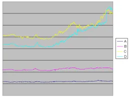
Figure 7 shows real stock data from four companies. From mined ratio rules among these 4 sequences, we find that sequence A and sequence B are independent with other sequences, while sequence C is related with se-quence D. We plot the data points of sequence A and sequence B in Figure 8, and we can verify that there is no linear relationship between sequence A and sequence

B. On the other hand, the data points of sequenceCand sequenceDare plotted in Figure 9, and we can mine ratio rules (in red solid segments) between the two sequence in terms of intervals of sequence C, as well as that in the last interval of sequence C, no linear relationship exists, and the real data of these two last subsequences are not similar with each other in Figure 7.

7

Conclusion

0 0.2 0.4 0.6 0.8 1 1.2

1 2 3 4 5 number of data points ex

ec ut io n tim e ra tio

Eigen-analysis based RARR Proposed approach

1000 2000 3000 4000 5000

(a) number of data points

0 0.2 0.4 0.6 0.8 1 1.2

1 2 3 4 5

number of data points

h-ho le g ue ss in g er ro ra tio

Eigen-analysis based RARR Proposed approach 1000 2000 3000 4000 5000 0

0.2 0.4 0.6 0.8 1 1.2

1 2 3 4 5

number of data points

h-ho le g ue ss in g er ro ra tio

Eigen-analysis based RARR Proposed approach 1000 2000 3000 4000 5000

[image:6.595.363.489.67.174.2]

(b) number of data points

[image:6.595.98.241.83.192.2]

Figure 6: Scalability analysis.

Figure 7: 4 real stock data sequences.

the nature of the pattern in the underlying data char-acteristics. Breaking the limitation of traditional batch process of eigen-analysis, we propose an incremental pro-cess for generating ratio rules. Innovation of theGR mea-surement addresses the problem for deriving ratio rules from subsets of data.

References

[1] Agrawal, R., Imielinski, T., Swami, A. N.: “Mining Association Rules between Sets of Items in Large

Databases“. ACM SIGMOD International

Confer-ence on Management of Data, Washington, D.C.pp.

207–216 93

[image:6.595.359.493.214.331.2]

[2] Korn, F., Labrinidis, A., Kotidis, Y., Faloutsos, C.:

Figure 8: Data sequenceAand data sequenceB.

Figure 9: Mined ratio rules between sequcenceC andD

in terms of trend intervals ofC.

“Quantifiable Data Mining Using Ratio Rules“.The

International Journal on Very Large Data Bases.

V8, N3-4, pp. 254–266. 00

[3] Hamamoto, M. and Kitagawa. H.: “Ratio Rules

Mining with Supprot and Confidence Factors“,

IEEE conference proceeding, pp. 500-505, 06

[4] Zhang, M., and Hsu, W., and Lee. M.: “Mining Prevalence-based Ratio Patterns“,IEEE conference proceeding, pp. 140-147, 07

[5] Yan, J., Liu, N., Yang, B. Y., Cheng, Q. S., Chen, Z.: “Mining Adaptive Ratio Rules from Distributed Data Sources“.Data Mining and Knowledge Discov-ery. V12, N2-3, pp. 249–273. 06

[6] Aggarwal, C.C.: “A Framework for Diagnosing

Changes in Evolving Data Streams“,ACM SIGMOD conference proceeding, pp. 575-786, 03

[7] Fan, W., Koyanagi, Y. S., Asakura, K.Y., Watan-abe T. H.: “An Incremental PCA for Stream Analy-sis Based on NLMS Adaptive Filter“. Tokai-Section Joint Conference on Electrical and Related Engi-neering, Aichi, O-511, 08

[8] Fan, W., Koyanagi, Y., Asakura, K., Watanabe. T.: “Generalized Regression Measure for Local Correla-tion Tracking in Evolving Data Streams“.1st Forum

on Data Engineering and Information Management.

[image:6.595.105.234.413.513.2]