Efficient Non parametric Estimation of Multiple Embeddings per Word in Vector Space

Efficient Non-parametric Estimation of

Multiple Embeddings per Word in Vector Space

Arvind Neelakantan*_{, Jeevan Shankar}*_{, Alexandre Passos, Andrew McCallum} Department of Computer Science

University of Massachusetts, Amherst Amherst, MA, 01003

{arvind,jshankar,apassos,mccallum}@cs.umass.edu

Abstract

There is rising interest in vector-space word embeddings and their use in NLP, especially given recent methods for their fast estimation at very large scale. Nearly all this work, however, assumes a sin-gle vector per word type—ignoring poly-semy and thus jeopardizing their useful-ness for downstream tasks. We present an extension to the Skip-gram model that efficiently learns multiple embeddings per word type. It differs from recent related work by jointly performing word sense discrimination and embedding learning, by non-parametrically estimating the num-ber of senses per word type, and by its ef-ficiency and scalability. We present new state-of-the-art results in the word similar-ity in context task and demonstrate its scal-ability by training with one machine on a corpus of nearly 1 billion tokens in less than 6 hours.

1 Introduction

Representing words by dense, real-valued vector embeddings, also commonly called “distributed representations,” helps address the curse of di-mensionality and improve generalization because they can place near each other words having sim-ilar semantic and syntactic roles. This has been shown dramatically in state-of-the-art results on language modeling (Bengio et al, 2003; Mnih and Hinton, 2007) as well as improvements in other natural language processing tasks (Collobert and Weston, 2008; Turian et al, 2010). Substantial benefit arises when embeddings can be trained on large volumes of data. Hence the recent consider-able interest in the CBOW and Skip-gram models

*_{The first two authors contributed equally to this paper.}

of Mikolov et al (2013a); Mikolov et al (2013b)— relatively simple log-linear models that can be trained to produce high-quality word embeddings on the entirety of English Wikipedia text in less than half a day on one machine.

There is rising enthusiasm for applying these models to improve accuracy in natural language processing, much like Brown clusters (Brown et al, 1992) have become common input features for many tasks, such as named entity extraction (Miller et al, 2004; Ratinov and Roth, 2009) and parsing (Koo et al, 2008; T¨ackstr¨om et al, 2012). In comparison to Brown clusters, the vector em-beddings have the advantages of substantially bet-ter scalability in their training, and intriguing po-tential for their continuous and multi-dimensional interrelations. In fact, Passos et al (2014) present new state-of-the-art results in CoNLL 2003 named entity extraction by directly inputting continuous vector embeddings obtained by a version of Skip-gram that injects supervision with lexicons. Sim-ilarly Bansal et al (2014) show results in depen-dency parsing using Skip-gram embeddings. They have also recently been applied to machine trans-lation (Zou et al, 2013; Mikolov et al, 2013c).

A notable deficiency in this prior work is that

each word type (e.g. the word string plant) has

only one vector representation—polysemy and hononymy are ignored. This results in the word

plant having an embedding that is approximately

the average of its different contextual seman-tics relating to biology, placement, manufactur-ing and power generation. In moderately high-dimensional spaces a vector can be relatively “close” to multiple regions at a time, but this does not negate the unfortunate influence of the triangle

inequality2_{here: words that are not synonyms but}

are synonymous with different senses of the same

word will be pulled together. For example,pollen

andrefinerywill be inappropriately pulled to a dis-2_{For distanced,d(a, c)≤d(a, b) +d(b, c).}

tance not more than the sum of the distancesplant– pollenandplant–refinery. Fitting the constraints of

legitimate continuous gradations of semantics are challenge enough without the additional encum-brance of these illegitimate triangle inequalities.

Discovering embeddings for multiple senses per word type is the focus of work by Reisinger and Mooney (2010a) and Huang et al (2012). They both pre-cluster the contexts of a word type’s to-kens into discriminated senses, use the clusters to re-label the corpus’ tokens according to sense, and then learn embeddings for these re-labeled words. The second paper improves upon the first by ploying an earlier pass of non-discriminated em-bedding learning to obtain vectors used to rep-resent the contexts. Note that by pre-clustering, these methods lose the opportunity to jointly learn the sense-discriminated vectors and the cluster-ing. Other weaknesses include their fixed num-ber of sense per word type, and the computational expense of the two-step process—the Huang et al (2012) method took one week of computation to learn multiple embeddings for a 6,000 subset of the 30,000 vocabulary on a corpus containing close to billion tokens.3

This paper presents a new method for learn-ing vector-space embeddlearn-ings for multiple senses per word type, designed to provide several ad-vantages over previous approaches. (1) Sense-discriminated vectors are learned jointly with the assignment of token contexts to senses; thus we can use the emerging sense representation to more accurately perform the clustering. (2) A non-parametric variant of our method automatically discovers a varying number of senses per word type. (3) Efficient online joint training makes it fast and scalable. We refer to our method as

Multiple-sense Skip-gram, orMSSG, and its

non-parametric counterpart asNP-MSSG.

Our method builds on the Skip-gram model (Mikolov et al, 2013a), but maintains multiple vectors per word type. During online training with a particular token, we use the average of its context words’ vectors to select the token’s sense that is closest, and perform a gradient update on that sense. In the non-parametric version of our

method, we build onfacility location (Meyerson,

2001): a new cluster is created with probability proportional to the distance from the context to the

3_{Personal communication with authors Eric H. Huang and} Richard Socher.

nearest sense.

We present experimental results demonstrating the benefits of our approach. We show quali-tative improvements over single-sense Skip-gram and Huang et al (2012), comparing against word neighbors from our parametric and non-parametric methods. We present quantitative results in three tasks. On both the SCWS and WordSim353 data sets our methods surpass the previous state-of-the-art. The Google Analogy task is not espe-cially well-suited for word-sense evaluation since its lack of context makes selecting the sense dif-ficult; however our method dramatically outper-forms Huang et al (2012) on this task. Finally we also demonstrate scalabilty, learning multiple senses, training on nearly a billion tokens in less than 6 hours—a 27x improvement on Huang et al.

2 Related Work

Much prior work has focused on learning vector representations of words; here we will describe only those most relevant to understanding this pa-per. Our work is based on neural language mod-els, proposed by Bengio et al (2003), which extend

the traditional idea ofn-gram language models by

replacing the conditional probability table with a neural network, representing each word token by a small vector instead of an indicator variable, and estimating the parameters of the neural network and these vectors jointly. Since the Bengio et al (2003) model is quite expensive to train, much re-search has focused on optimizing it. Collobert and Weston (2008) replaces the max-likelihood char-acter of the model with a max-margin approach, where the network is encouraged to score the

cor-rectn-grams higher than randomly chosen

incor-rect n-grams. Mnih and Hinton (2007) replaces

the global normalization of the Bengio model with a tree-structured probability distribution, and also considers multiple positions for each word in the tree.

downstream tasks. Neural networks or log-linear models also do not appear to be necessary to learn high-quality word embeddings, as Dhillon and Ungar (2011) estimate word vector repre-sentations using Canonical Correlation Analysis (CCA).

Word vector representations or embeddings have been used in various NLP tasks such as named entity recognition (Neelakantan and Collins, 2014; Passos et al, 2014; Turian et al, 2010), dependency parsing (Bansal et al, 2014), chunking (Turian et al, 2010; Dhillon and Ungar, 2011), sentiment analysis (Maas et al, 2011), para-phrase detection (Socher et al, 2011) and learning representations of paragraphs and documents (Le and Mikolov, 2014). The word clusters obtained from Brown clustering (Brown et al, 1992) have similarly been used as features in named entity recognition (Miller et al, 2004; Ratinov and Roth, 2009) and dependency parsing (Koo et al, 2008), among other tasks.

There is considerably less prior work on learn-ing multiple vector representations for the same word type. Reisinger and Mooney (2010a) intro-duce a method for constructing multiple sparse, high-dimensional vector representations of words. Huang et al (2012) extends this approach incor-porating global document context to learn mul-tiple dense, low-dimensional embeddings by us-ing recursive neural networks. Both the meth-ods perform word sense discrimination as a pre-processing step by clustering contexts for each word type, making training more expensive. While methods such as those described in Dhillon and Ungar (2011) and Reddy et al (2011) use token-specific representations of words as part of the learning algorithm, the final outputs are still one-to-one mappings between word types and word embeddings.

3 Background: Skip-gram model

The Skip-gram model learns word embeddings such that they are useful in predicting the sur-rounding words in a sentence. In the Skip-gram

model,v(w) ∈ Rd_{is the vector representation of}

the wordw ∈W, whereW is the words

vocabu-lary anddis the embedding dimensionality.

Given a pair of words (wt, c), the probability

that the wordcis observed in the context of word

wtis given by,

P(D= 1|v(wt), v(c)) = _{1 +e−v}1_(wt)T_v(c) (1)

The probability of not observing wordcin the

con-text ofwtis given by,

P(D= 0|v(wt), v(c)) =

1−P(D= 1|v(wt), v(c))

Given a training set containing the sequence of word typesw1, w2, . . . , wT, the word embeddings are learned by maximizing the following objective function:

J(θ) = X

(wt,ct)∈D+

X

c∈ct

logP(D= 1|v(wt), v(c))

+ X

(wt,c0t)∈D−

X

c0_∈c0

t

logP(D= 0|v(wt), v(c0))

where wt is the tth word in the training set, ct

is the set of observed context words of word wt

andc0

tis the set of randomly sampled, noisy

con-text words for the word wt. D+ consists of

the set of all observed word-context pairs(wt, ct) (t = 1,2. . . , T). D− _{consists of pairs (wt, c}0

t) (t = 1,2. . . , T) wherec0

t is the set of randomly

sampled, noisy context words for the wordwt.

For each training word wt, the set of context

wordsct ={wt−Rt, . . . , wt−1, wt+1, . . . , wt+Rt}

includesRtwords to the left and right of the given

word as shown in Figure 1. Rtis the window size

considered for the word wt uniformly randomly

sampled from the set {1,2, . . . , N}, where N is the maximum context window size.

The set of noisy context wordsc0

t for the word

wtis constructed by randomly sampling S noisy

context words for each word in the contextct. The

noisy context words are randomly sampled from the following distribution,

P(w) = punigram_Z(w)3/4 (2)

wherepunigram(w)is the unigram distribution of

the words andZis the normalization constant.

4 Multi-Sense Skip-gram (MSSG) model

Word Vector

word w

t

v(w

t+2)

Context Vectors

v(w_t+1)

v(w_t-1)

v(w

t-2)

v(w

t)

Figure 1: Architecture of the Skip-gram model

with window size Rt = 2. Context ct of word

wtconsists ofwt−1, wt−2, wt+1, wt+2.

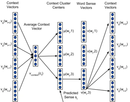
and let each sense of word have its own embed-ding, and induce the senses by clustering the em-beddings of the context words around each token. The vector representation of the context is the av-erage of its context words’ vectors. For every word type, we maintain clusters of its contexts and the sense of a word token is predicted as the cluster that is closest to its context representation. After predicting the sense of a word token, we perform a gradient update on the embedding of that sense. The crucial difference from previous approaches is that word sense discrimination and learning em-beddings are performed jointly by predicting the sense of the word using the current parameter es-timates.

In the MSSG model, each word w ∈ W is

associated with a global vector vg(w) and each

sense of the word has an embedding (sense vec-tor)vs(w, k)(k= 1,2, . . . , K) and a context clus-ter with cenclus-terµ(w, k)(k= 1,2, . . . , K). TheK

sense vectors and the global vectors are of

dimen-siondandKis a hyperparameter.

Consider the word wt and let ct =

{wt−Rt, . . . , wt−1, wt+1, . . . , wt+Rt} be the

set of observed context words. The vector repre-sentation of the context is defined as the average of the global vector representation of the words in the context. Letvcontext(ct) = _2∗1_RtPc∈ctvg(c)

be the vector representation of the contextct. We

use the global vectors of the context words instead of its sense vectors to avoid the computational complexity associated with predicting the sense

of the context words. We predict st, the sense

Word Sense Vectors

v(wt,2)

vg(wt+2)

Context Vectors

v_g(w_t+1)

vg(wt-1)

vg(wt-2)

Average Context Vector

Context Cluster Centers

v(wt,1)

v(wt,3)

Predicted Sense s_t μ(wt,1)

vcontext(ct)

μ(w_t,2)

μ(wt,3)

Context Vectors

vg(wt+2)

vg(wt+1)

vg(wt-1)

vg(wt-2)

Figure 2: Architecture of Multi-Sense Skip-gram

(MSSG) model with window size Rt = 2 and

K = 3. Context ct of word wt consists of

wt−1, wt−2, wt+1, wt+2. The sense is predicted by

finding the cluster center of the context that is clos-est to the average of the context vectors.

of word wt when observed with context ct as

the context cluster membership of the vector

vcontext(ct)as shown in Figure 2. More formally,

st= arg max

k=1,2,...,Ksim(µ(wt, k), vcontext(ct)) (3)

The hard cluster assignment is similar to the k

-means algorithm. The cluster center is the aver-age of the vector representations of all the contexts

which belong to that cluster. Forsimwe use

co-sine similarity in our experiments.

Here, the probability that the wordcis observed

in the context of word wt given the sense of the

wordwtis,

P(D= 1|st,vs(wt,1), . . . , vs(wt, K), vg(c))

=P(D= 1|vs(wt, st), vg(c))

= 1

1 +e−vs(wt,st)Tvg(c)

The probability of not observing wordcin the

con-text ofwtgiven the sense of the wordwtis,

P(D= 0|st,vs(wt,1), . . . , vs(wt, K), vg(c))

=P(D= 0|vs(wt, st), vg(c))

= 1−P(D= 1|vs(wt, st), vg(c))

Given a training set containing the sequence of

word typesw1, w2, ..., wT, the word embeddings

Algorithm 1Training Algorithm of MSSG model

1: Input:w₁, w₂, ..., w_T,d,K,N.

2: Initializev_s(w, k) andv_g(w), ∀w ∈ W, k ∈ {1, . . . , K}randomly,µ(w, k)∀w ∈ W, k ∈ {1, . . . , K}to 0.

3: fort= 1,2, . . . , T do 4: R_t∼ {1, . . . , N}

5: ct={wt−Rt, . . . , wt−1, wt+1, . . . , wt+Rt}

6: v_context(c_t) = _2∗1_RtP_c∈ctv_g(c) 7: s_t= arg max_k=1,2,...,K {

sim(µ(wt, k), vcontext(ct))}

8: Update context cluster center µ(w_t, s_t)

since contextctis added to context clusterst of wordwt.

9: c0_t=Noisy Samples(c_t)

10: Gradient update onv_s(w_t, s_t), global

vec-tors of words inctandc0t.

11: end for

12: Output: v_s(w, k), v_g(w) and context cluster

centersµ(w, k),∀w∈W, k∈ {1, . . . , K}

function:

J(θ) =

X

(wt,ct)∈D+

X

c∈ct

logP(D= 1|vs(wt, st), vg(c))+ X

(wt,c0t)∈D−

X

c0_∈c0

t

logP(D= 0|vs(wt, st), vg(c0))

wherewtis thetthword in the sequence,ctis the

set of observed context words andc0

t is the set of

noisy context words for the wordwt.D+andD−

are constructed in the same way as in the Skip-gram model.

After predicting the sense of word wt, we

up-date the embedding of the predicted sense for the wordwt(vs(wt, st)), the global vector of the words in the context and the global vector of the randomly sampled, noisy context words. The

con-text cluster center of cluster st for the word wt

(µ(wt, st)) is updated since contextctis added to the clusterst.

5 Non-Parametric MSSG model (NP-MSSG)

The MSSG model learns a fixed number of senses per word type. In this section, we describe a non-parametric version of MSSG, the NP-MSSG model, which learns varying number of senses per word type. Our approach is closely related to

the online non-parametric clustering procedure de-scribed in Meyerson (2001). We create a new clus-ter (sense) for a word type with probability propor-tional to the distance of its context to the nearest cluster (sense).

Each wordw∈W is associated with sense

vec-tors, context clusters and a global vectorvg(w)as in the MSSG model. The number of senses for a word is unknown and is learned during training. Initially, the words do not have sense vectors and context clusters. We create the first sense vector and context cluster for each word on its first occur-rence in the training data. After creating the first context cluster for a word, a new context cluster and a sense vector are created online during train-ing when the word is observed with a context were the similarity between the vector representation of the context with every existing cluster center of the

word is less than λ, where λis a hyperparameter

of the model.

Consider the word wt and let ct =

{wt−Rt, . . . , wt−1, wt+1, . . . , wt+Rt} be the

set of observed context words. The vector repre-sentation of the context is defined as the average of the global vector representation of the words in the context. Letvcontext(ct) = _2∗1_RtPc∈ctvg(c)

be the vector representation of the contextct. Let

k(wt) be the number of context clusters or the

number of senses currently associated with word

wt. st, the sense of wordwt whenk(wt) > 0is given by

st=     

k(wt) + 1, ifmaxk=1,2,...,k(wt){sim (µ(wt, k), vcontext(ct))}< λ

kmax, otherwise

(4)

where µ(wt, k) is the cluster center of

the kth _{cluster of word wt and kmax =}

arg max_{k=1,2,...,k(wt)}sim(µ(wt, k), vcontext(ct)). The cluster center is the average of the vector representations of all the contexts which belong to

that cluster. If st = k(wt) + 1, a new context

cluster and a new sense vector are created for the wordwt.

Model Time (in hours)

Huang et al 168

MSSG 50d 1

MSSG-300d 6

NP-MSSG-50d 1.83

NP-MSSG-300d 5

Skip-gram-50d 0.33

Skip-gram-300d 1.5

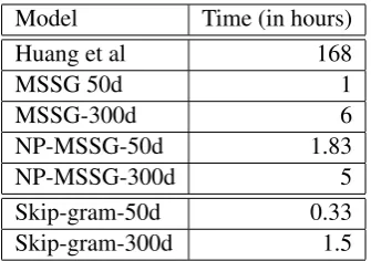
Table 1: Training Time Results. First five model reported in the table are capable of learning mul-tiple embeddings for each word and Skip-gram is capable of learning only single embedding for each word.

6 Experiments

To evaluate our algorithms we train embeddings using the same corpus and vocabulary as used in Huang et al (2012), which is the April 2010 snap-shot of the Wikipedia corpus (Shaoul and West-bury, 2010). It contains approximately 2 million articles and 990 million tokens. In all our experi-ments we remove all the words with less than 20 occurrences and use a maximum context window

(N) of length 5 (5 words before and after the word

occurrence). We fix the number of senses (K) to

be 3 for the MSSG model unless otherwise speci-fied. Our hyperparameter values were selected by a small amount of manual exploration on a

vali-dation set. In NP-MSSG we set λ to -0.5. The

Skip-gram model, MSSG and NP-MSSG models

sample one noisy context word (S) for each of the

observed context words. We train our models us-ing AdaGrad stochastic gradient decent (Duchi et al, 2011) with initial learning rate set to 0.025. Similarly to Huang et al (2012), we don’t use a regularization penalty.

Below we describe qualitative results, display-ing the embedddisplay-ings and the nearest neighbors of each word sense, and quantitative experiments in two benchmark word similarity tasks.

Table 1 shows time to train our models, com-pared with other models from previous work. All these times are from single-machine implementa-tions running on similar-sized corpora. We see that our model shows significant improvement in the training time over the model in Huang et al (2012), being within well within an order-of-magnitude of the training time for Skip-gram mod-els.

APPLE

Skip-gram blackberry, macintosh, acorn, pear, plum

MSSG pear, honey, pumpkin, potato, nutmicrosoft, activision, sony, retail, gamestop macintosh, pc, ibm, iigs, chipsets

NP-MSSG apricot, blackberry, cabbage, blackberries, pear_{microsoft, ibm, wordperfect, amiga, trs-80} FOX

Skip-gram abc, nbc, soapnet, espn, kttv

MSSG beaver, wolf, moose, otter, swannbc, espn, cbs, ctv, pbs dexter, myers, sawyer, kelly, griffith NP-MSSG rabbit, squirrel, wolf, badger, stoat_{cbs,abc, nbc, wnyw, abc-tv} NET

Skip-gram profit, dividends, pegged, profits, nets

MSSG snap, sideline, ball, game-trying, scoringnegative, offset, constant, hence, potential pre-tax, billion, revenue, annualized, us$

NP-MSSG

negative, total, transfer, minimizes, loop pre-tax, taxable, per, billion, us$, income ball, yard, fouled, bounced, 50-yard wnet, tvontorio, cable, tv, tv-5 ROCK

Skip-gram glam, indie, punk, band, pop

MSSG rocks, basalt, boulders, sand, quartzitealternative, progressive, roll, indie, blues-rock rocks, pine, rocky, butte, deer

NP-MSSG granite, basalt, outcropping, rocks, quartzite_{alternative, indie, pop/rock, rock/metal, blues-rock} RUN

Skip-gram running, ran, runs, afoul, amok

MSSG running, stretch, ran, pinch-hit, runsoperated , running, runs, operate, managed running, runs, operate, drivers, configure

NP-MSSG

two-run, walk-off, runs, three-runs, starts operated, runs, serviced, links, walk running, operating, ran, go, configure

re-election, reelection, re-elect, unseat, term-limited helmed, longest-running, mtv, promoted, produced

Table 2: Nearest neighbors of each sense of each word, by cosine similarity, for different algo-rithms. Note that the different senses closely cor-respond to intuitions regarding the senses of the given word types.

6.1 Nearest Neighbors

Skip-gram plants, flowering, weed, fungus, biomass MS

-SG

plants, tubers, soil, seed, biomass

refinery, reactor, coal-fired, factory, smelter asteraceae, fabaceae, arecaceae, lamiaceae, eri-caceae

NP MS -SG

plants, seeds, pollen, fungal, fungus

factory, manufacturing, refinery, bottling, steel fabaceae, legume, asteraceae, apiaceae, flowering power, coal-fired, hydro-power, hydroelectric, re-finery

Hua -ng et al

insect, capable, food, solanaceous, subsurface robust, belong, pitcher, comprises, eagles food, animal, catching, catch, ecology, fly seafood, equipment, oil, dairy, manufacturer facility, expansion, corporation, camp, co. treatment, skin, mechanism, sugar, drug facility, theater, platform, structure, storage natural, blast, energy, hurl, power

matter, physical, certain, expression, agents vine, mute, chalcedony, quandong, excrete

Table 3: Nearest Neighbors of the word plant

for different models. We see that the discovered senses in both our models are more semantically coherent than Huang et al (2012) and NP-MSSG is able to learn reasonable number of senses.

6.2 Word Similarity

We evaluate our embeddings on two related datasets: the WordSim-353 (Finkelstein et al, 2001) dataset and the Contextual Word Similari-ties (SCWS) dataset Huang et al (2012).

WordSim-353 is a standard dataset for evaluat-ing word vector representations. It consists of a list of pairs of word types, the similarity of which is rated in an integral scale from 1 to 10. Pairs include both monosemic and polysemic words. These scores to each word pairs are given with-out any contextual information, which makes them tricky to interpret.

To overcome this issue, Stanford’s Contextual Word Similarities (SCWS) dataset was developed by Huang et al (2012). The dataset consists of 2003 word pairs and their sentential contexts. It consists of 1328 noun-noun pairs, 399 verb-verb pairs, 140 verb-noun, 97 adjective-adjective, 30 noun-adjective, 9 verb-adjective, and 241 same-word pairs. We evaluate and compare our embed-dings on both WordSim-353 and SCWS word sim-ilarity corpus.

Since it is not trivial to deal with multiple em-beddings per word, we consider the following

sim-ilarity measures between words w and w0 _given

their respective contextscandc0_{, whereP(w, c, k)}

is the probability thatwtakes thekth _{sense given}

the contextc, andd(vs(w, i), vs(w0, j))is the sim-ilarity measure between the given embeddings

vs(w, i)andvs(w0, j). TheavgSimmetric,

avgSim(w, w0₎

= _K1₂

K X

i=1

K X

j=1

d(vs(w, i), vs(w0, j)),

computes the average similarity over all embed-dings for each word, ignoring information from the context.

To address this, theavgSimCmetric,

avgSimC(w, w0_{) =}XK

j=1

K X

i=1

P(w, c, i)P(w0_{, c}0_{, j)}

×d(vs(w, i), vs(w0, j))

weighs the similarity between each pair of senses by how well does each sense fit the context at hand.

The globalSimmetric uses each word’s global context vector, ignoring the many senses:

globalSim(w, w0_{) =d(v}

g(w), vg(w0)).

Finally, localSim metric selects a single sense

for each word based independently on its context and computes the similarity by

localSim(w, w0_{) =d(v}

s(w, k), vs(w0, k0)),

where k = arg max_iP(w, c, i) and k0 ₌

arg maxjP(w0, c0, j) and P(w, c, i) is the

prob-ability thatwtakes theith _{sense given contextc.}

The probability of being in a cluster is calculated as the inverse of the cosine distance to the cluster center (Huang et al, 2012).

We report the Spearman correlation between a model’s similarity scores and the human judge-ments in the datasets.

Model globalSim avgSim avgSimC localSim

TF-IDF 26.3 - -

-Collobort & Weston-50d 57.0 - -

-Skip-gram-50d 63.4 - -

-Skip-gram-300d 65.2 - -

-Pruned TF-IDF 62.5 60.4 60.5

-Huang et al-50d 58.6 62.8 65.7 26.1

MSSG-50d 62.1 64.2 66.9 49.17

MSSG-300d 65.3 67.2 69.3 57.26

NP-MSSG-50d 62.3 64.0 66.1 50.27

NP-MSSG-300d 65.5 67.3 69.1 59.80

Table 4: Experimental results in the SCWS task. The numbers are Spearmans correlation ρ ×100

between each model’s similarity judgments and the human judgments, in context. First three models

learn only a single embedding per model and hence,avgSim,avgSimCandlocalSimare not reported

for these models, as they’d be identical toglobalSim. Both our parametric and non-parametric models

outperform the baseline models, and our best model achieves a score of 69.3 in this task. NP-MSSG

achieves the best results whenglobalSim,avgSimandlocalSimsimilarity measures are used. The best

results according to each metric are in bold face.

Model ρ×100

HLBL 33.2

C&W 55.3

Skip-gram-300d 70.4

Huang et al-G 22.8

Huang et al-M 64.2

MSSG 50d-G 60.6

MSSG 50d-M 63.2

MSSG 300d-G 69.2

MSSG 300d-M 70.9

NP-MSSG 50d-G 61.5

NP-MSSG 50d-M 62.4

NP-MSSG 300d-G 69.1

NP-MSSG 300d-M 68.6

Pruned TF-IDF 73.4

ESA 75

Tiered TF-IDF 76.9

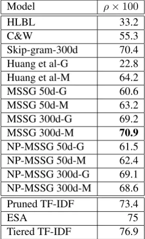
Table 5: Results on the WordSim-353 dataset.

The table shows the Spearmans correlation ρ

be-tween the model’s similarities and human

judg-ments. G indicates theglobalSimsimilarity

mea-sure and M indicates avgSim measure.The best

results among models that learn low-dimensional and dense representations are in bold face. Pruned TF-IDF (Reisinger and Mooney, 2010a), ESA (Gabrilovich and Markovitch, 2007) and Tiered TF-IDF (Reisinger and Mooney, 2010b) construct spare, high-dimensional representations.

Figure 3: The plot shows the distribution of num-ber of senses learned per word type in NP-MSSG model

given with their context, our model achieves new state-of-the-art results on SCWS as shown in the Table-4. The previous state-of-art model (Huang

et al, 2012) on this task achieves 65.7% using

the avgSimC measure, while the MSSG model

achieves the best score of69.3%on this task. The

results on the other metrics are similar. For a fixed embedding dimension, the model by Huang et al (2012) has more parameters than our model since it uses a hidden layer. The results show that our model performs better than Huang et al (2012) even when both the models use 50 dimen-sional vectors and the performance of our model improves as we increase the number of dimensions to 300.

(a) (b)

Figure 4: Figures (a) and (b) show the effect of varying embedding dimensionality and number of senses respectively of the MSSG Model on the SCWS task.

Model Task Sim ρ×100

Skip-gram WS-353 globalSim 70.4

MSSG WS-353 globalSim 68.4

MSSG WS-353 avgSim 71.2

NP MSSG WS-353 globalSim 68.3

NP MSSG WS-353 avgSim 69.66

MSSG SCWS localSim 59.3 MSSG SCWS globalSim 64.7 MSSG SCWS avgSim 67.2 MSSG SCWS avgSimC 69.2

NP MSSG SCWS localSim 60.11

NP MSSG SCWS globalSim 65.3

NP MSSG SCWS avgSim 67

NP MSSG SCWS avgSimC 68.6

Table 6: Experiment results on WordSim-353 and SCWS Task. Multiple Embeddings are learned for top 30,000 most frequent words in the vocabulary. The embedding dimension size is 300 for all the models for this task. The number of senses for MSSG model is 3.

introduced by Mikolov et al (2013a) where both MSSG and NP-MSSG models achieve 64% accu-racy compared to 12% accuaccu-racy by Huang et al (2012). Skip-gram which is the state-of-art model for this task achieves 67% accuracy.

Figure 3 shows the distribution of number of senses learned per word type in the NP-MSSG model. We learn the multiple embeddings for the same set of approximately 6000 words that were used in Huang et al (2012) for all our experiments

to ensure fair comparision. These approximately 6000 words were choosen by Huang et al. mainly from the top 30,00 frequent words in the vocab-ulary. This selection was likely made to avoid the noise of learning multiple senses for infre-quent words. However, our method is robust to noise, which can be seen by the good performance of our model that learns multiple embeddings for the top 30,000 most frequent words. We found that even by learning multiple embeddings for the top 30,000 most frequent words in the vocubu-lary, MSSG model still achieves state-of-art result

on SCWS task with anavgSimCscore of 69.2 as

shown in Table 6.

7 Conclusion

We present an extension to the Skip-gram model that efficiently learns multiple embeddings per word type. The model jointly performs word sense discrimination and embedding learning, and non-parametrically estimates the number of senses per word type. Our method achieves new state-of-the-art results in the word similarity in con-text task and learns multiple senses, training on close to billion tokens in less than 6 hours. The global vectors, sense vectors and cluster centers of our model and code for learning them are

avail-able at https://people.cs.umass.edu/

˜arvind/emnlp2014wordvectors. In

Acknowledgments

This work was supported in part by the Center for Intelligent Information Retrieval and in part by DARPA under agreement number FA8750-13-2-0020. The U.S. Government is authorized to re-produce and distribute reprints for Governmental purposes notwithstanding any copyright notation thereon. Any opinions, findings and conclusions or recommendations expressed in this material are those of the authors and do not necessarily reflect those of the sponsor.

References

Mohit Bansal, Kevin Gimpel, and Karen Livescu. 2014. Tailoring Continuous Word Representations for Dependency Parsing. Association for Computa-tional Linguistics (ACL).

Yoshua Bengio, R´ejean Ducharme, Pascal Vincent, and Christian Jauvin. 2003. A neural probabilistic lan-guage model. Journal of Machine Learning Re-search (JMLR).

Peter F. Brown, Peter V. Desouza, Robert L. Mercer, Vincent J. Della Pietra, and Jenifer C. Lai. 1992.

Class-based N-gram models of natural language

Computational Linguistics.

Ronan Collobert and Jason Weston. 2008. A Uni-fied Architecture for Natural Language Process-ing: Deep Neural Networks with Multitask Learn-ing. International Conference on Machine learning (ICML).

Paramveer S. Dhillon, Dean Foster, and Lyle Ungar. 2011.Multi-View Learning of Word Embeddings via CCA. Advances in Neural Information Processing Systems (NIPS).

John Duchi, Elad Hazan, and Yoram Singer 2011.

Adaptive sub- gradient methods for online learn-ing and stochastic optimization. Journal of Machine Learning Research (JMLR).

Lev Finkelstein, Evgeniy Gabrilovich, Yossi Matias, Ehud Rivlin, Zach Solan, Gadi Wolfman, and Eytan Ruppin. 2001. Placing search in context: the con-cept revisited. International Conference on World Wide Web (WWW).

Evgeniy Gabrilovich and Shaul Markovitch. 2007.

Computing semantic relatedness using wikipedia-based explicit semantic analysis. International Joint Conference on Artificial Intelligence (IJCAI). Eric H. Huang, Richard Socher, Christopher D.

Man-ning, and Andrew Y. Ng. 2012. Improving Word Representations via Global Context and Multiple Word Prototypes. Association of Computational Linguistics (ACL).

Terry Koo, Xavier Carreras, and Michael Collins. 2008.Simple Semi-supervised Dependency Parsing.

Association for Computational Linguistics (ACL).

Quoc V. Le and Tomas Mikolov. 2014 Distributed Representations of Sentences and Documents. Inter-national Conference on Machine Learning (ICML)

Andrew L. Maas, Raymond E. Daly, Peter T. Pham, Dan Huang, Andrew Y. Ng, and Christopher Potts. 2011 Learning Word Vectors for Sentiment Analysis

Association for Computational Linguistics (ACL)

Adam Meyerson. 2001 IEEE Symposium on Foun-dations of Computer Science. International Confer-ence on Machine Learning (ICML)

Tomas Mikolov, Kai Chen, Greg Corrado, and Jef-frey Dean. 2013a. Efficient Estimation of Word Representations in Vector Space. Workshop at In-ternational Conference on Learning Representations (ICLR).

Tomas Mikolov, Ilya Sutskever, Kai Chen, Greg Cor-rado, and Jeffrey Dean. 2013b. Distributed Repre-sentations of Words and Phrases and their Composi-tionality. Advances in Neural Information Process-ing Systems (NIPS).

Tomas Mikolov, Quoc V. Le, and Ilya Sutskever. 2013c. Exploiting Similarities among Languages for Machine Translation. arXiv.

Scott Miller, Jethran Guinness, and Alex Zamanian. 2004. Name tagging with word clusters and dis-criminative training. North American Chapter of the Association for Computational Linguistics: Hu-man Language Technologies (NAACL-HLT).

Andriy Mnih and Geoffrey Hinton. 2007. Three new graphical models for statistical language mod-elling. International Conference on Machine learn-ing (ICML).

Arvind Neelakantan and Michael Collins. 2014.

Learning Dictionaries for Named Entity Recogni-tion using Minimal Supervision. European Chap-ter of the Association for Computational Linguistics (EACL).

Alexandre Passos, Vineet Kumar, and Andrew McCal-lum. 2014. Lexicon Infused Phrase Embeddings for Named Entity Resolution. Conference on Natural Language Learning (CoNLL).

Lev Ratinov and Dan Roth. 2009. Design Chal-lenges and Misconceptions in Named Entity Recog-nition. Conference on Natural Language Learning (CoNLL).

Joseph Reisinger and Raymond J. Mooney. 2010a.

Multi-prototype vector-space models of word mean-ing. North American Chapter of the Association for Computational Linguistics: Human Language Tech-nologies (NAACL-HLT)

Joseph Reisinger and Raymond Mooney. 2010b. A mixture model with sharing for lexical semantics.

Empirical Methods in Natural Language Processing (EMNLP).

Cyrus Shaoul and Chris Westbury. 2010.The Westbury lab wikipedia corpus.

Richard Socher, Eric H. Huang, Jeffrey Pennington, Andrew Y. Ng, and Christopher D. Manning. 2011

Dynamic Pooling and Unfolding Recursive Autoen-coders for Paraphrase Detection. Advances in Neu-ral Information Processing Systems (NIPS). Oscar T¨ackstr¨om, Ryan McDonald, and Jakob

Uszkor-eit. 2012. Cross-lingual Word Clusters for Direct Transfer of Linguistic Structure. North American Chapter of the Association for Computational Lin-guistics: Human Language Technologies.

Joseph Turian, Lev Ratinov, and Yoshua Bengio. 2010.Word Representations: A Simple and General Method for Semi-Supervised Learning. Association for Computational Linguistics (ACL).