Discriminative Neural Sentence Modeling by Tree Based Convolution

Discriminative Neural Sentence Modeling

by Tree-Based Convolution

Lili Mou∗_{, Hao Peng}∗_{, Ge Li}†_{, Yan Xu, Lu Zhang, Zhi Jin}

{doublepower.mou, penghao.pku}@gmail.com

{lige, xuyan14, zhanglu, zhijin}@sei.pku.edu.cn Software Institute, Peking University, 100871, P. R. China

Abstract

This paper proposes a tree-based con-volutional neural network (TBCNN) for discriminative sentence modeling. Our model leverages either constituency trees or dependency trees of sentences. The tree-based convolution process extracts sentences structural features, which are then aggregated by max pooling. Such ar-chitecture allows short propagation paths between the output layer and underlying feature detectors, enabling effective struc-tural feature learning and extraction. We evaluate our models on two tasks: senti-ment analysis and question classification. In both experiments, TBCNN outperforms previous state-of-the-art results, including existing neural networks and dedicated feature/rule engineering. We also make efforts to visualize the tree-based convo-lution process, shedding light on how our models work.

1 Introduction

Discriminative sentence modeling aims to capture sentence meanings, and classify sentences accord-ing to certain criteria (e.g., sentiment). It is related to various tasks of interest, and has attracted much attention in the NLP community (Allan et al., 2003; Su and Markert, 2008; Zhao et al., 2015). Feature engineering—for example, n-gram tures (Cui et al., 2006), dependency subtree fea-tures (Nakagawa et al., 2010), or more dedicated ones (Silva et al., 2011)—can play an important role in modeling sentences. Kernel machines, e.g., SVM, are exploited in Moschitti (2006) and Re-ichartz et al. (2010) by specifying a certain mea-sure of similarity between sentences, without ex-plicit feature representation.

∗_{These authors contribute equally to this paper.} †_{To whom correspondence should be addressed.}

Recent advances of neural networks bring new techniques in understanding natural languages, and have exhibited considerable potential. Bengio et al. (2003) and Mikolov et al. (2013) propose un-supervised approaches to learn word embeddings, mapping discrete words to real-valued vectors in a meaning space. Le and Mikolov (2014) ex-tend such approaches to learn sentences’ and para-graphs’ representations. Compared with human engineering, neural networks serve as a way of au-tomatic feature learning (Bengio et al., 2013).

Two widely used neural sentence models are convolutional neural networks (CNNs) and recur-sive neural networks (RNNs). CNNs can extract words’ neighboring features effectively with short propagation paths, but they do not capture inher-ent sinher-entence structures (e.g., parse trees). RNNs encode, to some extent, structural information by recursive semantic composition along a parse tree. However, they may have difficulties in learning deep dependencies because of long propagation paths (Erhan et al., 2009). (CNNs/RNNs and a variant, recurrent networks, will be reviewed in Section 2.)

A curious question is whether we can com-bine the advantages of CNNs and RNNs, i.e., whether we can exploit sentence structures (like RNNs) effectively with short propagation paths (like CNNs).

In this paper, we propose a novel neural ar-chitecture for discriminative sentence modeling, called theTree-Based Convolutional Neural Net-work(TBCNN).1_{Our models can leverage} differ-ent sdiffer-entence parse trees, e.g., constituency trees and dependency trees. The model variants are de-noted as c-TBCNN and d-TBCNN, respectively. The idea of tree-based convolution is to apply a set of subtree feature detectors, sliding over the entire

1_{The model of tree-based convolution was firstly}

pro-posed to process program source code in our (unpublished) previous work (Mou et al., 2014).

1

x … xt

Embeddings

W Extracted

features by convolution Pooling layer Output layer

Word embeddings

Softmax

Representing hidden layers as vectors recursively

l

W

r

W

Parsing tree of a sentence

Max pooling by heuristics

Hidden Output layer layer

Softmax

Softmax

l

W

r

W

(a) CNN (b) RNN (c) TBCNN

Extracted features by tree-based convolution

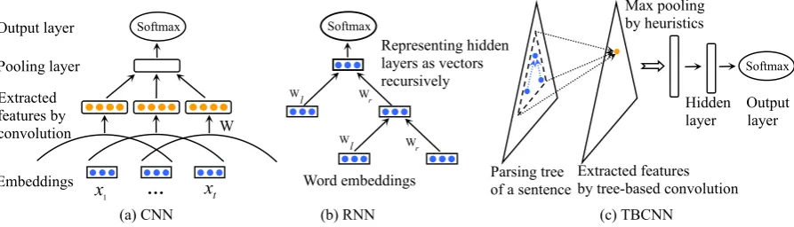
Figure 1: A comparison of information flow in the convolutional neural network (CNN), the recursive neural network (RNN), and the tree-based convolutional neural network (TBCNN).

parse tree of a sentence; then pooling aggregates these extracted feature vectors by taking the max-imum value in each dimension. One merit of such architecture is that all features, along the tree, have short propagation paths to the output layer, and hence structural information can be learned effec-tively.

TBCNNs are evaluated on two tasks, sentiment analysis and question classification; our models have outperformed previous state-of-the-art re-sults in both experiments. To understand how TBCNNs work, we also visualize the network by plotting the convolution process. We make our code and results available on our project website.2

2 Background and Related Work

In this section, we present the background and re-lated work regarding two prevailing neural archi-tectures for discriminative sentence modeling.

2.1 Convolutional Neural Networks

Convolutional neural networks (CNNs), early used for image processing (LeCun, 1995), turn out to be effective with natural languages as well. Figure 1a depicts a classic convolution process on a sentence (Collobert and Weston, 2008). A set of fixed-width-window feature detectors slide over the sentence, and output the extracted features. Let

t be the window size, andx1,· · · ,xt ∈ Rne be ne-dimensional word embeddings. The output of

convolution, evaluated at the current position, is

y=f(W ·[x1;· · · ;xt] +b)

wherey∈Rnc (n_cis the number of feature

detec-tors). W ∈ Rnc×(t·ne) andb ∈ Rnc are parame-2_{https://sites.google.com/site/tbcnnsentence/}

ters;f is the activation function. Semicolons rep-resent column vector concatenation. After convo-lution, the extracted features are pooled to a fixed-size vector for classification.

Convolution can extract neighboring informa-tion effectively. However, the features are “local”—words that are not in a same convolu-tion window do not interact with each other, even though they may be semantically related. Blun-som et al. (2014) build deep convolutional net-works so that local features can mix at high-level layers. Similar CNNs include Kim (2014) and Hu et al. (2014). All these models are “flat,” by which we mean no structural information is used explic-itly.

2.2 Recursive Neural Networks

Recursive neural networks (RNNs), proposed in Socher et al. (2011b), utilize sentence parse trees. In the original version, RNN is built upon a binarized constituency tree. Leaf nodes corre-spond to words in a sentence, represented byne

-dimensional embeddings. Non-leaf nodes are sen-tence constituents, coded by child nodes recur-sively. Let nodepbe the parent ofc1 andc2, vec-tor representations denoted asp,c1, andc2. The parent’s representation is composited by

Im-provements for semantic compositionality include matrix-vector interaction (Socher et al., 2012), tensor interaction (Socher et al., 2013). They are more suitable for capturing logical information in sentences, such as negation and exclamation.

One potential problem of RNNs is that the long propagation paths—through which leaf nodes are connected to the output layer—may lead to infor-mation loss. Thus, RNNs bury illuminating in-formation under a complicated neural architecture. Further, during back-propagation over a long path, gradients tend to vanish (or blow up), which makes training difficult (Erhan et al., 2009). Long short term memory (LSTM), first proposed for model-ing time-series data (Hochreiter and Schmidhuber, 1997), is integrated to RNNs to alleviate this prob-lem (Tai et al., 2015; Le and Zuidema, 2015; Zhu et al., 2015).

Recurrent networks. A variant class of RNNs is the recurrent neural network (Bengio et al., 1994; Shang et al., 2015), whose architecture is a rightmost tree. In such models, meaningful tree structures are also lost, similar to CNNs.

3 Tree-based Convolution

This section introduces the proposed tree-based convolutional neural networks (TBCNNs). Figure 1c depicts the convolution process on a tree.

First, a sentence is converted to a parse tree, ei-ther a constituency or dependency tree. The corre-sponding model variants are denoted as c-TBCNN and d-TBCNN. Each node in the tree is repre-sented as a distributed, real-valued vector.

Then, we design a set of fixed-depth subtree fea-ture detectors, called the tree-based convolution window. The window slides over the entire tree to extract structural information of the sentence, illustrated by a dashed triangle in Figure 1c. For-mally, let us assume we have tnodes in the con-volution window,x1,· · · ,xt, each represented as

an ne-dimensional vector. Let nc be the number

of feature detectors. The output of the tree-based convolution window, evaluated at the current sub-tree, is given by the following generic equation.

y=f t

X

i=1

Wi·xi+b

!

(2)

whereWi ∈Rnc×ne is the weight parameter

asso-ciated with nodexi;b∈Rnc is the bias term.

Extracted features are thereafter packed into one or more fixed-size vectors by max pooling,

that is, the maximum value in each dimension is taken. Finally, we add a fully connected hidden layer, and asoftmaxoutput layer.

From the designed architecture (Figure 1c), we see that our TBCNN models allow short propaga-tion paths between the output layer and any posi-tion in the tree. Therefore structural feature learn-ing becomes effective.

Several main technical points in tree-based con-volution include: (1) How can we represent hid-den nodes as vectors in constituency trees? (2) How can we determine weights, Wi, for

depen-dency trees, where nodes may have different num-bers of children? (3) How can we pool varying sized and shaped features to fixed-size vectors?

In the rest of this section, we explain model variants in detail. Particularly, Subsections 3.1 and 3.2 address the first and second problems; Sub-section 3.3 deals with the third problem by intro-ducing several pooling heuristics. Subsection 3.4 presents our training objective.

3.1 c-TBCNN

Figure 2a illustrates an example of the con-stituency tree, where leaf nodes are words in the sentence, and non-leaf nodes represent a grammat-ical constituent, e.g., a noun phrase. Sentences are parsed by the Stanford parser;3 _further, con-stituency trees are binarized for simplicity.

One problem of constituency trees is that non-leaf nodes do not have such vector representations as word embeddings. Our strategy is to pretrain the constituency tree with an RNN by Equation 1 (Socher et al., 2011b). After pretraining, vector representations of nodes are fixed.

We now consider the tree-based convolution process in c-TBCNN with a two-layer-subtree convolution window, which operates on a parent nodepand its direct childrenclandcr, their

vec-tor representations denoted asp, cl, andcr. The

convolution equation, specific for c-TBCNN, is

y=fW(c)

p ·p+Wl(c)·cl+Wr(c)·cr+b(c)

where Wp(c), W_l(c), and Wr(c) are weights

asso-ciated with the parent and its child nodes. Su-perscript (c) indicates that the weights are for c-TBCNN. For leaf nodes, which do not have chil-dren, we setclandcrto be0.

I

it loved

Constituency tree Dependency tree

it

Extracted features by c-TBCNN

Extracted features by d-TBCNN

(a) (b)

loved

nsubj dobj

I

Figure 2: Tree-based convolution in (a) c-TBCNN, and (b) d-TBCNN. The parse trees correspond to the sentence “I loved it.” The dashed triangles illustrate a shared-weight convolution window sliding over the tree. For clarity, only two positions are drawn in c-TBCNN. Notice that dotted arrows are not part of neural connections; they merely indicate the topologies of tree structures. Specially, an edgea→r bin the dependency tree refers toabeing governed bybwith dependency typer.

Tree-based convolution windows can be ex-tended to arbitrary depths straightforwardly. The complexity is exponential to the depth of the window, but linear to the number of nodes. Hence, tree-based convolution, compared with “flat” CNNs, does not add to computational cost, provided the same amount of information to pro-cess at a time. In our experiments, we use convo-lution windows of depth 2.

3.2 d-TBCNN

Dependency trees are another representation of sentence structures. The nature of dependency representation leads to d-TBCNN’s major dif-ference from traditional convolution: there ex-ist nodes with different numbers of child nodes. This causes trouble if we associate weight param-eters according to positions in the window, which is standard for traditional convolution, e.g., Col-lobert and Weston (2008) or c-TBCNN.

To overcome the problem, we extend the no-tion of convoluno-tion by assigning weights accord-ing to dependency types (e.g,nsubj) rather than positions. We believe this strategy makes much sense because dependency types (de Marneffe et al., 2006) reflect the relationship between a gov-erning word and its child words. To be concrete, the generic convolution formula (Equation 2) for d-TBCNN becomes

y=f W(d)

p ·p+

n

X

i=1

W_r(_[d_c)_i]·ci+b(d)

!

where Wp(d) is the weight parameter for the

par-ent p (governing word); W_r(_[d_c)_i] is the weight for child ci, who has grammatical relationship r[ci]

… …

Each slot chooses the maximum value in a dimension

kpooling slots (k= 2) (a) Global pooling (b) 3-slot pooling for c-TBCNN

GLOBAL

LEFT RIGHT TOP

Extracted features by tree-based convolution in the order of words LOWER LOWER

(c)k-slot pooling for d-TBCNN

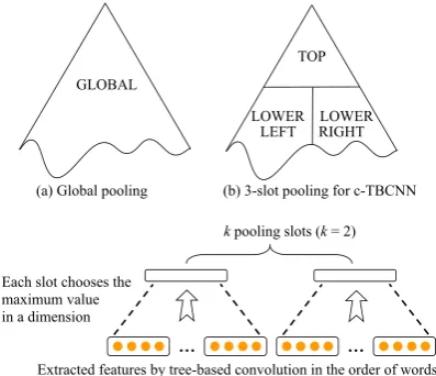
Figure 3: Pooling heuristics. (a) Global pooling. (b) 3-slot pooling for c-TBCNN. (c)k-slot pooling for d-TBCNN.

to its parent, p. Superscript(d)indicates the pa-rameters are for d-TBCNN. Note that we keep 15 most frequently occurred dependency types; oth-ers appearing rarely in the corpus are mapped to one shared weight matrix.

Both c-TBCNN and d-TBCNN have their own advantages: d-TBCNN exploits structural features more efficiently because of the compact expres-siveness of dependency trees; c-TBCNN may be more effective in integrating global features due to the underneath pretrained RNN.

3.3 Pooling Heuristics

Task Data samples Label Sentiment

Analysis

Offers that rare combination of entertainment and education. ++

An idealistic love story that brings out the latent 15-year-old romantic in everyone. +

Its mysteries are transparently obvious, and it’s too slowly paced to be a thriller. − Question

Classification What is the temperature at the center of the earth?What state did the Battle of Bighorn take place in? locationnumber

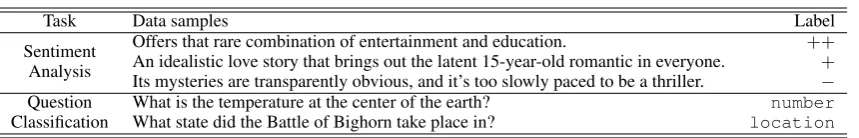
Table 1: Data samples in sentiment analysis and question classification. In the first task, “++” refers to strongly positive; “+” and “−” refer to positive and negative, respectively.

this problem. We propose several heuristics for pooling along a tree structure. Our generic de-sign criteria for pooling include: (1) Nodes that are pooled to one slot should be “neighboring” from some viewpoint. (2) Each slot should have similar numbers of nodes, in expectation, that are pooled to it. Thus, (approximately) equal amount of information is aggregated along different parts of the tree. Following the above intuition, we pro-pose pooling heuristics as follows.

• Global pooling. All features are pooled to one vector, shown in Figure 3a. We take the maximum value in each dimension. This simple heuristic is applicable to any structure, including c-TBCNN and d-TBCNN.

• 3-slot pooling for c-TBCNN. To preserve more information over different parts of con-stituency trees, we propose 3-slot pooling (Figure 3b). If a tree has maximum depth

d, we pool nodes of less than α · d lay-ers to a TOP slot (α is set to 0.6); lower nodes are pooled to slots LOWER LEFT or LOWER RIGHT according to their relative position with respect to the root node. For a constituency tree, it is not completely obvious how to pool features to more than 3 slots and comply with the aforementioned criteria at the same time. Therefore, we re-gard 3-slot pooling for c-TBCNN is a “hard mechanism” temporarily. Further improve-ment can be addressed in future work. • k-slot pooling for d-TBCNN. Different from

constituency trees, nodes in dependency trees are one-one corresponding to words in a sen-tence. Thus, a total order on features (af-ter convolution) can be defined according to their corresponding word orders. For k -slot pooling, we can adopt an “equal allo-cation” strategy, shown in Figure 3c. Let

i be the position of a word in a sentence (i = 1,2,· · · , n). Its extracted feature vec-tor is pooled to thej-th slot, if

(j−1)n_k ≤i≤jn_k

We assess the efficacy of pooling quantitatively in Section 4.3.1. As we shall see by the exper-imental results, complicated pooling methods do preserve more information along tree structures to some extent, but the effect is not large. TBCNNs are not very sensitive to pooling methods.

3.4 Training Objective

After pooling, information is packed into one or more fixed-size vectors (slots). We add a hidden layer, and then asoftmaxlayer to predict the prob-ability of each target label in a classification task. The error function of a sample is the standard cross entropy loss, i.e.,J =−Pc_i=1tilogyi, wheretis

the ground truth (one-hot represented),ythe out-put bysoftmax, andcthe number of classes. To regularize our model, we apply both`2penalty and dropout (Srivastava et al., 2014). Training details are further presented in Section 4.1 and 4.2.

4 Experimental Results

In this section, we evaluate our models with two tasks, sentiment analysis and question classifica-tion. We also conduct quantitative and qualitative model analysis in Subsection 4.3.

4.1 Sentiment Analysis 4.1.1 The Task and Dataset

Sentiment analysis is a widely studied task for discriminative sentence modeling. The Stanford sentiment treebank4_{consists of more than 10,000} movie reviews. Two settings are considered for sentiment prediction: (1) fine-grained classifi-cation with 5 labels (strongly positive, positive, neutral, negative, and strongly negative), and (2) coarse-gained polarity classification with 2 labels (positive versusnegative). Some examples are shown in

Table 1. We use the standard split for training, val-idating, and testing, containing 8544/1101/2210 sentences for 5-class prediction. Binary classifi-cation does not contain theneutralclass.

In the dataset, phrases (sub-sentences) are also tagged with sentiment labels. RNNs deal with them naturally during the recursive process. We regard sub-sentences as individual samples during training, like Blunsom et al. (2014) and Le and Mikolov (2014). The training set therefore has more than 150,000 entries in total. For validating and testing, only whole sentences (root labels) are considered in our experiments.

Both c-TBCNN and d-TBCNN use the Stanford parser for data preprocessing.

4.1.2 Training Details

This subsection describes training details for d-TBCNN, where hyperparameters are chosen by validation. c-TBCNN is mostly tuned syn-chronously (e.g., optimization algorithm, activa-tion funcactiva-tion) with some changes in hyperparam-eters. c-TBCNN’s settings can be found on our website.

In our d-TBCNN model, the number of units is 300 for convolution and 200 for the last hid-den layer. Word embeddings are 300 dimensional, pretrained ourselves using word2vec (Mikolov et al., 2013) on the English Wikipedia corpus. 2-slot pooling is applied for d-TBCNN. (c-TBCNN uses 3-slot pooling.)

To train our model, we compute gradient by back-propagation and apply stochastic gradient descent with mini-batch 200. We useReLU(Nair and Hinton, 2010) as the activation function .

For regularization, we add `2 penalty for weights with a coefficient of10−5_{. Dropout} (Sri-vastava et al., 2014) is further applied to both weights and embeddings. All hidden layers are dropped out by 50%, and embeddings 40%.

4.1.3 Performance

Table 2 compares our models to state-of-the-art results in the task of sentiment analysis. For 5-class prediction, d-TBCNN yields 51.4% accu-racy, outperforming the previous state-of-the-art result, achieved by the RNN based on long-short term memory (Tai et al., 2015). c-TBCNN is slightly worse. It achieves 50.4% accuracy, rank-ing third in the state-of-the-art list (includrank-ing our d-TBCNN model).

Regarding 2-class prediction, we adopted a sim-ple strategy in Irsoy and Cardie (2014),5_{where the} 5-class network is “transferred” directly for binary classification, with estimated target probabilities (by 5-way softmax) reinterpreted for 2 classes. (Theneutralclass is discarded as in other stud-ies.) This strategy enables us to take a glance at the stability of our TBCNN models, but places itself in a difficult position. Nonetheless, our d-TBCNN model achieves 87.9% accuracy, ranking forth in the list.

In a more controlled comparison—with shal-low architectures and the basic interaction (lin-early transformed and non-lin(lin-early squashed)— TBCNNs, of both variants, consistently outper-form RNNs (Socher et al., 2011b) to a large ex-tent (50.4–51.4% versus 43.2%); they also con-sistently outperform “flat” CNNs by more than 10%. Such results show that structures are im-portant when modeling sentences; tree-based con-volution can capture these structural information more effectively than RNNs.

We also observe d-TBCNN achieves higher per-formance than c-TBCNN. This suggests that com-pact tree expressiveness is more important than in-tegrating global information in this task.

4.2 Question Classification

We further evaluate TBCNN models on a ques-tion classificaques-tion task.6 _{The dataset contains} 5452 annotated sentences plus 500 test sam-ples in TREC 10. We also use the stan-dard split, like Silva et al. (2011). Target la-bels contain 6 classes, namelyabbreviation, entity,description, human, location, andnumeric. Some examples are also shown in Table 1.

We chose this task to evaluate our models be-cause the number of training samples is rather small, so that we can know TBCNNs’ perfor-mance when applied to datasets of different sizes. To alleviate the problem of data sparseness, we set the dimensions of convolutional layer and the last hidden layer to 30 and 25, respectively. We do not back-propagate gradient to embeddings in this

5_{Richard Socher, who first applies neural networks to this}

task, thinks direct transfer is fine for binary classification. We followed this strategy for simplicity as it is non-trivial to deal with the neutral sub-sentences in the training set if we train a separate model. Our website reviews some related work and provides more discussions.

Group Method 5-class accuracy 2-class accuracy Reported in

Baseline _{Na¨ıve Bayes}SVM 40.7_41.0 79.4_81.8 Socher et al. (2013)_{Socher et al. (2013)}

CNNs

1-layer convolution 37.4 77.1 Blunsom et al. (2014)

Deep CNN 48.5 86.8 Blunsom et al. (2014)

Non-static 48.0 87.2 Kim (2014)

Multichannel 47.4 88.1 Kim (2014)

RNNs

Basic 43.2 82.4 Socher et al. (2013)

Matrix-vector 44.4 82.9 Socher et al. (2013)

Tensor 45.7 85.4 Socher et al. (2013)

Tree LSTM (variant 1) 48.0 – Zhu et al. (2015) Tree LSTM (variant 2) 51.0 88.0 Tai et al. (2015) Tree LSTM (variant 3) 49.9 88.0 Le and Zuidema (2015)

Deep RNN 49.8 86.6† _{Irsoy and Cardie (2014)}

Recurrent _bi-LSTMLSTM 45.8_49.1 86.7_86.8 Tai et al. (2015)_{Tai et al. (2015)} Vector Word vector avg._{Paragraph vector} 32.7_48.7 80.1_87.8 Socher et al. (2013)_{Le and Mikolov (2014)} TBCNNs c-TBCNN_d-TBCNN 50.4_51.4 86.8_87.9†_† Our implementation_{Our implementation}

Table 2: Accuracy of sentiment prediction (in percentage). For 2-class prediction, “†” remarks indicate that the network is transferred directly from that of 5-class.

Method Acc.(%) Reported in

SVM _{95.0 Silva et al. (2011)} 10k features + 60 rules

CNN-non-static 93.6 Kim (2014) CNN-mutlichannel 92.2 Kim (2014)

RNN 90.2 Zhao et al. (2015) Deep-CNN 93.0 Blunsom et al. (2014)

Ada-CNN 92.4 Zhao et al. (2015) c-TBCNN 94.8 Our implementation d-TBCNN 96.0 Our implementation Table 3: Accuracy of 6-way question classification.

task. Dropout rate for embeddings is 30%; hidden layers are dropped out by 5%.

Table 3 compares our models to various other methods. The first entry presents the previous state-of-the-art result, achieved by traditional fea-ture/rule engineering (Silva et al., 2011). Their method utilizes more than 10k features and 60 hand-coded rules. On the contrary, our TBCNN models do not use a single human-engineered fea-ture or rule. Despite this, c-TBCNN achieves similar accuracy compared with feature engineer-ing; d-TBCNN pushes the state-of-the-art result to 96%. To the best of our knowledge, this is the first time that neural networks beat dedicated human engineering in this question classification task.

The result also shows that both c-TBCNN and d-TBCNN reduce the error rate to a large extent, compared with other neural architectures in this task.

4.3 Model Analysis

In this part, we analyze our models quantitatively and qualitatively in several aspects, shedding some light on the mechanism of TBCNNs.

4.3.1 The Effect of Pooling

The extracted features by tree-based convolution have topologies varying in size and shape. We pro-pose in Section 3.3 several heuristics for pooling. This subsection aims to provide a fair comparison among these pooling methods.

One reasonable protocol for comparison is to tune all hyperparameters for each setting and com-pare the highest accuracy. This methodology, however, is too time-consuming, and depends largely on the quality of hyperparameter tuning. An alternative is to predefine a set of sensible hy-perparameters and report the accuracy under the same setting. In this experiment, we chose the latter protocol, where hidden layers are all 300-dimensional; no`2 penalty is added. Each config-uration was run five times with different random initializations. We summarize the mean and stan-dard deviation in Table 4.

Model Pooling method 5-class accuracy (%)

c-TBCNN Global_3-slot 48.48_48.69±_±0.54_0.40 d-TBCNN Global_2-slot 49.39_49.94±_±0.24_0.63

Table 4: Accuracies of different pooling methods, averaged over 5 random initializations. We chose sensible hyperparameters manually in advance to make a fair comparison. This leads to performance degradation (1–2%) vis-a-vis Table 2.

≤9 10−14 15−19 20−24 25−29 30−34 ≥35

Setence length

0

10

20

30

40

50

Accuracy (%)

RNN

c-TBCNN

d-TBCNN

Figure 4: Accuracies versus sentence lengths.

Comparing with other studies in the literature, we also notice that pooling is very effective and ef-ficient in information gathering. Irsoy and Cardie (2014) report 200 epochs for training a deep RNN, which achieves 49.8% accuracy in the 5-class sen-timent classification. Our TBCNNs are typically trained within 25 epochs.

4.3.2 The Effect of Sentence Lengths

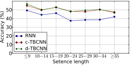
We analyze how sentence lengths affect our mod-els. Sentences are split into 7 groups by length, with granularity 5. A few too long or too short sentences are grouped together for smoothing; the numbers of sentences in each group vary from 126 to 457. Figure 4 presents accuracies versus lengths in TBCNNs. For comparison, we also reimple-mented RNN, achieving 42.7% overall accuracy, slightly worse than 43.2% reported in Socher et al. (2011b). Thus, we think our reimplementation is fair and that the comparison is sensible.

We observe that c-TBCNN and d-TBCNN yield very similar behaviors. They consistently outper-form the RNN in all scenarios. We also notice the gap, between TBCNNs and RNN, increases when sentences contain more than 20 words. This re-sult confirms our theoretical analysis in Section 2—for long sentences, the propagation paths in RNNs are deep, causing RNNs’ difficulty in in-formation processing. By contrast, our models ex-plore structural information more effectively with

tree-based convolution. As information from any part of the tree can propagate to the output layer with short paths, TBCNNs are more capable for sentence modeling, especially for long sentences. 4.3.3 Visualization

Visualization is important to understanding the mechanism of neural networks. For TBCNNs, we would like to see how the extracted features (af-ter convolution) are further processed by the max pooling layer, and ultimately related to the super-vised task.

To show this, we trace back where the max pooling layer’s features come from. For each di-mension, the pooling layer chooses the maximum value from the nodes that are pooled to it. Thus, we can count the fraction in which a node’s fea-tures are gathered by pooling. Intuitively, if a node’s features are more related to the task, the fraction tends to be larger, and vice versa.

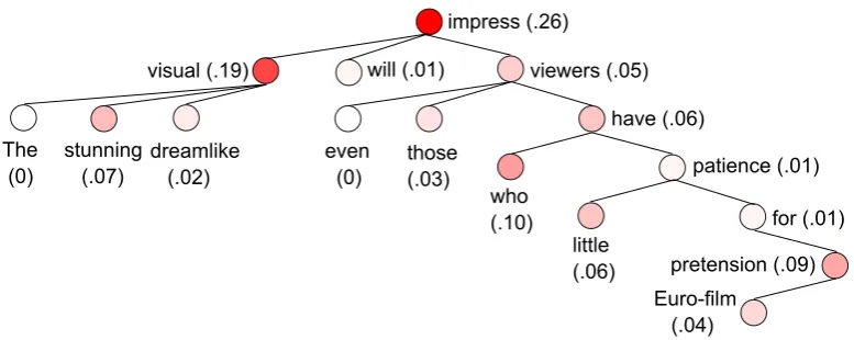
Figure 5 illustrates an example processed by d-TBCNN in the task of sentiment analysis.7 _Here, we applied global pooling because information tracing is more sensible with one pooling slot. As shown in the figure, tree-based convolution can effectively extract information relevant to the task of interest. The 2-layer windows correspond-ing to “visual will impress viewers,” “the stunning dreamlike visual,” say, are discriminative to the sentence’s sentiment. Hence, large fractions (0.24 and 0.19) of their features, after convolution, are gathered by pooling. On the other hand, words likethe,will,evenare known as stop words (Fox, 1989). They are mostly noninformative for sen-timent; hence, no (or minimal) features are gath-ered. Such results are consistent with human intu-ition.

We further observe that tree-based convolution does integrate information of different words in the window. For example, the wordstunning ap-pears in two windows: (a) the window “stunning” itself, and (b) the window of “the stunning dream-like visual,” with root nodevisual,stunningacting as a child. We see that Window b is more rel-evant to the ultimate sentiment than Window a, with fractions 0.19 versus 0.07, even though the root visual itself is neutral in sentiment. In fact,

7_{We only have space to present one example in the paper.}

The c(0)

stunning ccc(.07)

dreamlike ccc(.02)

visualc(.19) willc(.01) viewersc(.05)

impressc(.26)

even cc(0)

those (.03)

havec(.06)

who (.10)

patiencec(.01)

little (.06)

forc(.01)

pretensionc(.09) Euro-film

ccc(.04)

Figure 5: Visualizing how features (after convolution) are related to the sentiment of a sentence. The sample corresponds a sentence in the dataset, “The stunning dreamlike visual will impress even those viewers who have little patience for Euro-film pretension.” The numbers in brackets denote the fraction of a node’s features that are gathered by the max pooling layer (also indicated by colors).

Windowahas a larger fraction than the sum of its children’s (the windows of “the,” “stunning,” and “dreamlike”).

5 Conclusion

In this paper, we proposed a novel neural discrim-inative sentence model based on sentence parsing structures. Our model can be built upon either constituency trees (denoted as c-TBCNN) or de-pendency trees (d-TBCNN).

Both variants have achieved high performance in sentiment analysis and question classification. d-TBCNN is slightly better than c-TBCNN in our experiments, and has outperformed previous state-of-the-art results in both tasks. The results show that tree-based convolution can capture sentences’ structural information effectively, which is useful for sentence modeling.

Acknowledgments

This research is supported by the National Basic Research Program of China (the 973 Program) un-der Grant No. 2015CB352201 and the National Natural Science Foundation of China under Grant Nos. 61232015 and 91318301.

References

James Allan, Courtney Wade, and Alvaro Bolivar. 2003. Retrieval and novelty detection at the sen-tence level. InProceedings of the 26th Annual Inter-national ACM SIGIR Conference on Research and Development in Informaion Retrieval, pages 314– 321. ACM.

Yoshua Bengio, Patrice Simard, and Paolo Frasconi. 1994. Learning long-term dependencies with gradi-ent descgradi-ent is difficult. IEEE Transactions on Neu-ral Networks, 5(2):157–166.

Yoshua Bengio, Rejean Ducharme, Pascal Vincent, and Christian Jauvin. 2003. A neural probabilistic lan-guage model. Journal of Machine Learning Re-search, 3:1137–1155.

Yoshua Bengio, Aaron Courville, and Pierre Vincent. 2013. Representation learning: A review and new perspectives. IEEE Transactions on Pattern Analy-sis and Machine Intelligence, 35(8):1798–1828.

Phil Blunsom, Edward Grefenstette, and Nal Kalch-brenner. 2014. A convolutional neural network for modelling sentences. In Proceedings of the 52nd Annual Meeting of the Association for Computa-tional Linguistics.

Ronan Collobert and Jason Weston. 2008. A unified architecture for natural language processing: Deep neural networks with multitask learning. In Pro-ceedings of the 25th International Conference on Machine learning, pages 160–167.

Hang Cui, Vibhu Mittal, and Mayur Datar. 2006. Comparative experiments on sentiment classifica-tion for online product reviews. In Proceedings 21st AAAI Conference on Artificial Intelligence, vol-ume 6, pages 1265–1270.

Marie-Catherine de Marneffe, Bill MacCartney, and Christopher D. Manning. 2006. Generating typed dependency parses from phrase structure parses. In Proceedings of Language Resource and Evaluation Conference, volume 6, pages 449–454.

effect of unsupervised pre-training. In Proceed-ings of International Conference on Artificial Intel-ligence and Statistics, pages 153–160.

Christopher Fox. 1989. A stop list for general text. In ACM SIGIR Forum, volume 24, pages 19–21.

Karl M. Hermann and Phil Blunsom. 2013. The role of syntax in vector space models of compositional semantics. InProceedings of the 51st Annual Meet-ing of the Association for Computational LMeet-inguis- Linguis-tics, pages 894–904.

Sepp Hochreiter and Jurgen Schmidhuber. 1997. Long short-term memory. Neural computation, 9(8):1735–1780.

Baotian Hu, Zhengdong Lu, Hang Li, and Qingcai Chen. 2014. Convolutional neural network archi-tectures for matching natural language sentences. InAdvances in Neural Information Processing Sys-tems, pages 2042–2050.

Ozan Irsoy and Claire Cardie. 2014. Deep recursive neural networks for compositionality in language. InAdvances in Neural Information Processing Sys-tems, pages 2096–2104.

Mohit Iyyer, Jordan Boyd-Graber, Leonardo Claudino, Richard Socher, and Hal Daum´e III. 2014. A neural network for factoid question answering over para-graphs. InProceedings of the 2014 Conference on Empirical Methods in Natural Language Process-ing, pages 633–644.

Yoon Kim. 2014. Convolutional neural networks for sentence classification. Proceedings of the 2014 Conference on Empirical Methods in Natural Lan-guage Processing.

Quoc V. Le and Tomas Mikolov. 2014. Distributed representations of sentences and documents. In Pro-ceedings of the 31st International Conference on Machine Learning.

Phong Le and Willem Zuidema. 2015. Compositional distributional semantics with long short term mem-ory.arXiv preprint arXiv:1503.02510.

Yann LeCun. 1995. Comparison of learning algo-rithms for handwritten digit recognition. In Pro-ceedings of International Conference on Artificial Neural Networks, volume 60, pages 53–60.

Tomas Mikolov, Ilya Sutskever, Kai Chen, Greg S. Cor-rado, and Jeff Dean. 2013. Distributed representa-tions of words and phrases and their compositional-ity. InAdvances in Neural Information Processing Systems, pages 3111–3119.

Alessandro Moschitti. 2006. Efficient convolution ker-nels for dependency and constituent syntactic trees. InProceedings of European Conference of Machine Learning, pages 318–329. Springer.

Lili Mou, Ge Li, Zhi Jin, Lu Zhang, and Tao Wang. 2014. TBCNN: A tree-based convolutional neu-ral network for programming language processing. arXiv preprint arXiv:1409.5718.

Vinod Nair and Geoffrey E. Hinton. 2010. Rectified linear units improve restricted Boltzmann machines. InProceedings of the 27th International Conference on Machine Learning, pages 807–814.

Tetsuji Nakagawa, Kentaro Inui, and Sadao Kurohashi. 2010. Dependency tree-based sentiment classifica-tion using CRFs with hidden variables. InHuman Language Technologies: The 2010 Annual Confer-ence of the North American Chapter of the Associa-tion for ComputaAssocia-tional Linguistics, pages 786–794.

Frank Reichartz, Hannes Korte, and Gerhard Paass. 2010. Semantic relation extraction with kernels over typed dependency trees. InProceedings of the 16th ACM SIGKDD International Conference on Knowl-edge Discovery and Data Mining, pages 773–782.

Lifeng Shang, Zhengdong Lu, and Hang Li. 2015. Neural responding machine for short-text conversa-tion. InProceedings of the 53rd Annual Meeting of the Association for Computational Linguistics and the 7th International Joint Conference on Natural Language Processing, pages 1577–1586.

Joao Silva, Lu´ısa Coheur, Ana C. Mendes, and Andreas Wichert. 2011. From symbolic to sub-symbolic in-formation in question classification. Artificial Intel-ligence Review, 35(2):137–154.

Richard Socher, Eric H. Huang, Jeffrey Pennin, Christopher D. Manning, and Andrew Y. Ng. 2011a. Dynamic pooling and unfolding recursive autoen-coders for paraphrase detection. In Advances in Neural Information Processing Systems, pages 801– 809.

Richard Socher, Jeffrey Pennington, Eric H. Huang, Andrew Y. Ng, and Christopher D. Manning. 2011b. Semi-supervised recursive autoencoders for predict-ing sentiment distributions. In Proceedings of the Conference on Empirical Methods in Natural Lan-guage Processing, pages 151–161.

Richard Socher, Brody Huval, Christopher D. Man-ning, and Andrew Y. Ng. 2012. Semantic composi-tionality through recursive matrix-vector spaces. In Proceedings of the 2012 Joint Conference on Empir-ical Methods in Natural Language Processing and Computational Natural Language Learning, pages 1201–1211.

Nitish Srivastava, Geoffrey Hinton, Alex Krizhevsky, Ilya Sutskever, and Ruslan Salakhutdinov. 2014. Dropout: A simple way to prevent neural networks from overfitting. Journal of Machine Learning Re-search, 15(1):1929–1958.

Fangzhong Su and Katja Markert. 2008. From words to senses: a case study of subjectivity recognition. InProceedings of the 22nd International Conference on Computational Linguistics-Volume 1, pages 825– 832. Association for Computational Linguistics. Kaisheng Tai, Richard Socher, and Christopher D.

Manning. 2015. Improved semantic representa-tions from tree-structured long short-term memory networks. InProceedings of the 53rd Annual Meet-ing of the Association for Computational LMeet-inguistics and the 7th International Joint Conference on Natu-ral Language Processing, pages 1556–1566. Han Zhao, Zhengdong Lu, and Pascal Poupart. 2015.

Self-adaptive hierarchical sentence model. In Pro-ceedings of the Twenty-Fourth International Joint Conference on Artificial Intelligence, pages 4069– 4076.