A Joint Segmentation and Classification Framework for Sentiment Analysis

A Joint Segmentation and Classification Framework

for Sentiment Analysis

Duyu Tang\∗_{, Furu Wei}‡_{, Bing Qin}\_{, Li Dong}]∗_{, Ting Liu}\_{, Ming Zhou}‡ \_{Research Center for Social Computing and Information Retrieval,}

Harbin Institute of Technology, China ‡_{Microsoft Research, Beijing, China} ]_{Beihang University, Beijing, China}

\_{{dytang, qinb, tliu}@ir.hit.edu.cn}

‡_{{fuwei, mingzhou}@microsoft.com} ]_{[email protected]}

Abstract

In this paper, we propose a joint segmenta-tion and classificasegmenta-tion framework for sen-timent analysis. Existing sensen-timent clas-sification algorithms typically split a sen-tence as a word sequence, which does not effectively handle the inconsistent senti-ment polarity between a phrase and the words it contains, such as “not bad” and

“a great deal of”. We address this issue

by developing a joint segmentation and classification framework (JSC), which si-multaneously conducts sentence segmen-tation and sentence-level sentiment classi-fication. Specifically, we use a log-linear model to score each segmentation candi-date, and exploit the phrasal information of top-ranked segmentations as features to build the sentiment classifier. A marginal log-likelihood objective function is de-vised for the segmentation model, which is optimized for enhancing the sentiment classification performance. The joint mod-el is trained only based on the annotat-ed sentiment polarity of sentences, with-out any segmentation annotations. Experi-ments on a benchmark Twitter sentimen-t classificasentimen-tion dasentimen-tasesentimen-t in SemEval 2013 show that, our joint model performs com-parably with the state-of-the-art methods.

1 Introduction

Sentiment classification, which classifies the senti-ment polarity of a sentence (or docusenti-ment) as posi-tive or negaposi-tive, is a major research direction in the field of sentiment analysis (Pang and Lee, 2008; Liu, 2012; Feldman, 2013). Majority of existing approaches follow Pang et al. (2002) and treat

sen-∗_{This work was partly done when the first and fourth}

authors were visiting Microsoft Research.

timent classification as a special case of text cate-gorization task. Under this perspective, previous studies typically use pipelined methods with two steps. They first produce sentence segmentation-s with segmentation-separate text analyzersegmentation-s (Choi and Cardie, 2008; Nakagawa et al., 2010; Socher et al., 2013b) or bag-of-words (Paltoglou and Thelwall, 2010; Maas et al., 2011). Then, feature learning and sen-timent classification algorithms take the segmenta-tion results as inputs to build the sentiment classi-fier (Socher et al., 2011; Kalchbrenner et al., 2014; Dong et al., 2014).

The major disadvantage of a pipelined method is the problem of error propagation, since sen-tence segmentation errors cannot be corrected by the sentiment classification model. A typical kind of error is caused by thepolarity inconsistency be-tween a phrase and the words it contains, such

as hnot bad, badi and ha great deal of, greati.

The segmentations based on bag-of-words or syn-tactic chunkers are not effective enough to han-dle thepolarity inconsistencyphenomenons. The reason lies in that bag-of-words segmentations re-gard each word as a separate unit, which losses the word order and does not capture the phrasal information. The segmentations based on syntac-tic chunkers typically aim to identify noun group-s, verb groups or named entities from a sentence. However, many sentiment indicators are phrases constituted of adjectives, negations, adverbs or id-ioms (Liu, 2012; Mohammad et al., 2013a), which are splitted by syntactic chunkers. Besides, a bet-ter approach would be to utilize the sentiment in-formation to improve the segmentor. Accordingly, the sentiment-specific segmentor will enhance the performance of sentiment classification in turn.

In this paper, we propose a joint segmentation and classification framework (JSC) for sentimen-t analysis, which simulsentimen-taneous conducsentimen-ts sensentimen-tence segmentation and sentence-level sentiment clas-sification. The framework is illustrated in

Segmentations Input

that is not bad

that is not bad that is not bad that is not bad that is not bad Polarity: +1

-1 -1 +1 +1

<+1,-1> NO

Polarity Update <+1,-1> NO

<+1,+1> YES

<+1,+1> YES

SC SEG

CG

Update SC

2.3 1.6

0.6 0.4

0.6 0.4 2.3 1.6 SEG

Rank

Top K

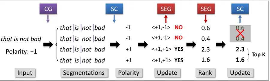
Figure 1: The joint segmentation and classification framework (JSC) for sentiment classification. CG

represents the candidate generation model,SCmeans the sentiment classification model andSEGstands for the segmentation ranking model. Down Arrowmeans the use of a specified model, andUp Arrow

indicates the update of a model.

ure 1. We develop (1) a candidate generation mod-el to generate the segmentation candidates of a sentence, (2) a segmentation ranking model to s-core each segmentation candidate of a given sen-tence, and (3) a classification model to predic-t predic-the senpredic-timenpredic-t polaripredic-ty of each segmenpredic-tapredic-tion. The phrasal information of top-ranked candidates from the segmentation model are utilized as features to build the sentiment classifier. In turn, the predict-ed sentiment polarity of segmentation candidates from classification model are leveraged to update the segmentor. We score each segmentation can-didate with a log-linear model, and optimize the segmentor with a marginal log-likelihood objec-tive. We train the joint model from sentences an-notated only with sentiment polarity, without any segmentation annotations.

We evaluate the effectiveness of our joint mod-el on a benchmark Twitter sentiment classifica-tion dataset in SemEval 2013. Results show that the joint model performs comparably with state-of-the-art methods, and consistently outperforms pipeline methods in various experiment settings. The main contributions of the work presented in this paper are as follows.

• To our knowledge, this is the first work that automatically produces sentence segmenta-tion for sentiment classificasegmenta-tion within a joint framework.

• We show that the joint model yields com-parable performance with the state-of-the-art methods on the benchmark Twitter sentiment classification datasets in SemEval 2013.

2 Related Work

Existing approaches for sentiment classification are dominated by two mainstream directions. Lexicon-based approaches (Turney, 2002; Ding et al., 2008; Taboada et al., 2011; Thelwall et al., 2012) typically utilize a lexicon of sentiment words, each of which is annotated with the sen-timent polarity or sensen-timent strength. Linguis-tic rules such as intensifications and negations are usually incorporated to aggregate the sentimen-t polarisentimen-ty of sensentimen-tences (or documensentimen-ts). Corpus-based methods treat sentiment classification as a special case of text categorization task (Pang et al., 2002). They mostly build the sentiment classifier from sentences (or documents) with manually an-notated sentiment polarity or distantly-supervised corpora collected by sentiment signals like emoti-cons (Go et al., 2009; Pak and Paroubek, 2010; Kouloumpis et al., 2011; Zhao et al., 2012).

between Naive Bayes and NB-feature enhanced SVM. Kim and Zhai (2009) and Paltoglou and Thelwall (2010) learn the feature weights by in-vestigating variants weighting functions from In-formation Retrieval. Nakagawa et al. (2010) uti-lize dependency trees, polarity-shifting rules and conditional random fields (Lafferty et al., 2001) with hidden variables to compute the documen-t feadocumen-ture. On Twidocumen-tdocumen-ter, Mohammad edocumen-t al. (2013b) develop a state-of-the-art Twitter sentiment classi-fier in SemEval 2013, using a variety of sentiment lexicons and hand-crafted features.

With the revival of deep learning (representa-tion learning (Hinton and Salakhutdinov, 2006; Bengio et al., 2013; Jones, 2014)), more recen-t srecen-tudies focus on learning recen-the low-dimensional, dense and real-valued vector as text features for sentiment classification. Glorot et al. (2011) inves-tigate Stacked Denoising Autoencoders to learn document vector for domain adaptation in sen-timent classification. Yessenalina and Cardie (2011) represent each word as a matrix and compose words using iterated matrix multipli-cation. Socher et al. propose Recursive Au-toencoder (RAE) (2011), Matrix-Vector Recursive Neural Network (MV-RNN) (2012) and Recur-sive Neural Tensor Network (RNTN) (2013b) to learn the composition of variable-length phrases based on the representation of its children. To learn the sentence representation, Kalchbrenner et al. (2014) exploit Dynamic Convolutional Neu-ral Network and Le and Mikolov (2014) inves-tigate Paragraph Vector. To learn word vectors for sentiment analysis, Maas et al. (2011) propose a probabilistic document model following Blei et al. (2003), Labutov and Lipson (2013) re-embed words from existing word embeddings and Tang et al. (2014b) develop three neural networks to learn word vectors from tweets containing posi-tive/negative emoticons.

Unlike most previous corpus-based algorithms that build sentiment classifier based on splitting a sentence as a word sequence, we produce sentence segmentations automatically within a joint frame-work, and conduct sentiment classification based on the segmentation results.

3 The Proposed Approach

In this section, we first give the task definition of two tasks, namely sentiment classification and sentence segmentation. Then, we present the

overview of the proposed joint segmentation and classification model (JSC) for sentiment analysis. The segmentation candidate generation model and the segmentation ranking model are described in Section 4. The details of the sentiment classifica-tion model are presented in Secclassifica-tion 5.

3.1 Task Definition

The task of sentiment classification has been well formalized in previous studies (Pang and Lee, 2008; Liu, 2012). The objective is to identify the sentiment polarity of a sentence (or document) as positive or negative1_.

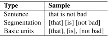
The task of sentence segmentation aims to s-plit a sentence into a sequence of exclusive part-s, each of which is a basic computational unit of the sentence. An example is illustrated in Table 1. The original text “that is not bad” is segmented

as “[that] [is] [not bad]”. The segmentation

re-sult is composed of three basic computational u-nits, namely[that],[is]and[not bad].

Type Sample

Sentence that is not bad Segmentation [that] [is] [not bad] Basic units [that], [is], [not bad]

Table 1: Example for sentence segmentation.

3.2 Joint Model (JSC)

The overview of the proposed joint segmentation and classification model (JSC) for sentiment anal-ysis is illustrated in Figure 1. The intuitions of the joint model are two-folds:

• The segmentation results have a strong influ-ence on the sentiment classification perfor-mance, since they are the inputs of the sen-timent classification model.

• The usefulness of a segmentation can be judged by whether the sentiment classifier can use it to predict the correct sentence po-larity.

Based on the mutual influence observation, we formalize the joint model in Algorithm 1. The in-puts contain two parts, training data and feature extractors. Each sentence si in the training data 1_{In this paper, the sentiment polarity of a sentence is not}

Algorithm 1The joint segmentation and classifi-cation framework (JSC) for sentiment analysis

Input:

training data:T = [si,polig],1≤i≤ |T|

segmentation feature extractor:sfe(·)

classification feature extractor:cfe(·) Output:

sentiment classifier:SC

segmentation ranking model:SEG

1: Generate segmentation candidatesΩ_ifor each

sentencesiinT,1≤i≤ |T|

2: Initialize sentiment classifierSC(0) based on

cfe(Ωij), randomize j ∈ [1,|Ωi|], 1 ≤ i ≤

|T|

3: Randomly initialize the segmentation ranking

modelSEG(0)

4: forr ←1... Rdo

5: Predict the sentiment polarity poli for Ωi

based onSC(r−1)_andcfe(Ω

i·)

6: Update the segmentation model SEG(r)

with SEG(r−1) _{and [Ωi, sfe(Ωi·),}

poli·, polgi],1≤i≤ |T| 7: fori←1...|T|do

8: Calculate the segmentation score forΩi·

based onSEG(r)_andsfe(Ω

i·)

9: Select the top-ranked K segmentation

candidatesΩi∗fromΩi 10: end for

11: Train the sentiment classifier SC(r) with

cfe(Ωi∗),1≤i≤ |T| 12: end for

13: SC←SC(R) 14: SEG←SEG(R)

T is annotated only with its gold sentiment po-laritypolg_i, without any segmentation annotation-s. There are two feature extractors for the task of sentence segmentation (sfe(·)) and sentiment classification (cfe(·)), respectively. The output-s of the joint model are the output-segmentation ranking modelSEGand the sentiment classifierSC.

In Algorithm 1, we first generate segmentation candidatesΩi for each sentencesi in the training

set (line 1). Each Ωi contains no less than one

segmentation candidates. We randomly select one segmentation result from eachΩiand utilize their

classification features to initialize the sentimen-t classifierSC(0) _{(line 2). We randomly initialize}

the segmentation model SEG(0) (line 3). Subse-quently, we iteratively train the segmentation

mod-elSEG(r)_{and sentiment classifierSC}(r)_{in a}

join-t manner (line 4-12). Ajoin-t each ijoin-terajoin-tion, we pre-dict the sentiment polarity of each segmentation candidateΩi· with the current sentiment

classifi-erSC(r−1) _{(line 5), and then leverage them to}

up-date the segmentation modelSEG(r)_{(line 6).}

Af-terwards, we utilize the recently updated segmen-tation ranking modelSEG(r) _{to update the}

senti-ment classifierSC(r) (line 7-11). We extract the segmentation features for each segmentation can-didateΩi·, and employ them to calculate the

seg-mentation score (line 8). The top-rankedK seg-mentation resultsΩi∗of each sentencesiis

select-ed (line 9), and further usselect-ed to train the sentimen-t classifierSC(r) (line 11). Finally, after training R iterations, we dump the segmentation ranking model SEG(R) _{and sentiment classifier SC}(R) _in

the last iteration as outputs (line 13-14).

At training time, we train the segmentation model and classification model from sentences with manually annotated sentiment polarity. At prediction time, given a test sentence, we gener-ate its segmentation candidgener-ates, and then calculgener-ate segmentation score for each candidate. Afterward-s, we select the top-rankedKcandidates and vote their predicted sentiment polarity from sentiment classifier as the final result.

4 Segmentation Model

In this section, we present details of the segmenta-tion candidate generasegmenta-tion model (Secsegmenta-tion 4.1), the segmentation ranking model (Section 4.2) and the feature description for segmentation ranking mod-el (Section 4.3).

4.1 Segmentation Candidate Generation

In this subsection, we describe the strategy to gen-erate segmentation candidates for each sentence. Since the segmentation results have an exponen-tial search space in the number of words in a sentence, we approximate the computation using beam search with constrains on a phrase table, which is induced from massive corpora.

Many studies have been previously proposed to recognize phrases in the text. However, it is out of scope of this work to compare them. We ex-ploit a data-driven approach given by Mikolov et al. (2013), which identifies phrases based on the occurrence frequency of unigrams and bigrams,

freq(wi, wj) = _freqfreq_(w(wi, wj)−δ

whereδ is a discounting coefficient that prevents too many phrases consisting of very infrequen-t words. We run 2-4 infrequen-times over infrequen-the corpora infrequen-to geinfrequen-t longer phrases containing more words. We em-pirically set δ as 10 in our experiment. We use the default frequency threshold (value=5) in the word2vec toolkit2_{to select bi-terms.}

Given a sentence, we initialize the beam of each index with the current word, and sequentially add phrases into the beam if the new phrase is con-tained in the phrase table. At each index of a sen-tence, we rank the segmentation candidates by the inverted number of items within a segmentation, and save the top-ranked N segmentation candi-dates into the beam. An example of the generated segmentation candidates is given in Table 2.

Type Sample

Sentence that is not bad

Phrase Table [is not], [not bad], [is not bad]

Segmentations

[that] [is not bad] [that] [is not] [bad] [that] [is] [not bad] [that] [is] [not] [bad]

Table 2: Example for segmentation candidate gen-eration.

4.2 Segmentation Ranking Model

The objective of the segmentation ranking model is to assign a scalar to each segmentation candi-date, which indicates the usefulness of the seg-mentation result for sentiment classification. In this subsection, we describe a log-linear model to calculate the segmentation score. To effectively train the segmentation ranking model, we devise a marginal log-likelihood as the optimization objec-tive.

Given a segmentation candidateΩij of the

sen-tence si, we calculate the segmentation score

forΩij with a log-linear model, as given in

Equa-tion 2.

φij =exp(b+X k

sfeijk·wk) (2)

whereφijis the segmentation score ofΩij;sfeijk

is thek-th segmentation feature ofΩij;wandbare

the parameters of the segmentation ranking model. During training, given a sentencesiand its gold

sentiment polarity polg_i, the optimization

objec-2_{Available at https://code.google.com/p/word2vec/}

tive of the segmentation ranking model is to max-imize the segmentation scores of the hit candi-dates, whose predicted sentiment polarity equal-s to the gold polarity of equal-sentencepol_ip. The loss function of the segmentation model is given in E-quation 3.

loss=−X|T|

i=1

log( P

j∈Hiφij

P

j0_∈Aiφ_ij0) +λ||w||

2

2 (3)

whereT is the training data;Airepresents all the

segmentation candidates of sentencesi;Hi

mean-s the hit candidatemean-s ofsi; λ is the weight of the

L2-norm regularization factor. We train the seg-mentation model with L-BFGS (Liu and Nocedal, 1989), running over the complete training data.

4.3 Feature

We design two kinds of features for sentence seg-mentation, namely the phrase-embedding feature and the segmentation-specific feature. The final feature representation of each segmentation is the concatenation of these two features. It is worth noting that, the phrase-embedding feature is used in both sentence segmentation and sentiment clas-sification.

Segmentation-Specific Feature We empirically design four segmentation-specific features to re-flect the information of each segmentation, as list-ed in Table 3.

Phrase-Embedding Feature We leverage phrase embedding to generate the features of segmentation candidates for both sentence seg-mentation and sentiment classification. The reason is that, in both tasks, the basic compu-tational units of each segmentation candidate might be words or phrases of variable length. Under this scenario, phrase embedding is highly suitable as it is capable to represent phrases with different length into a consistent distributed vector space (Mikolov et al., 2013). For each phrase, phrase embedding is a dense, real-valued and continuous vector. After the phrase embedding is trained, the nearest neighbors in the embedding space are favored to have similar grammatical us-ages and semantic meanings. The effectiveness of phrase embedding has been verified for building large-scale sentiment lexicon (Tang et al., 2014a) and machine translation (Zhang et al., 2014).

state-of-Feature Feature Description

#unit the number of basic computation units in the segmentation candidate #unit/#word the ratio of units’ number in a candidate to the length of original sentence

#word−#unit the difference between sentence length and the number of basic computational units #unit>2 the number of basic component units composed of more than two words

Table 3: Segmentation-specific features for segmentation ranking.

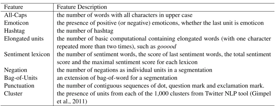
Feature Feature Description

All-Caps the number of words with all characters in upper case

Emoticon the presence of positive (or negative) emoticons, whether the last unit is emoticon

Hashtag the number of hashtag

Elongated units the number of basic computational containing elongated words (with one character repeated more than two times), such asgooood

Sentiment lexicon the number of sentiment words, the score of last sentiment words, the total sentiment score and the maximal sentiment score for each lexicon

Negation the number of negations as individual units in a segmentation Bag-of-Units an extension of bag-of-word for a segmentation

Punctuation the number of contiguous sequences of dot, question mark and exclamation mark. Cluster the presence of units from each of the 1,000 clusters from Twitter NLP tool (Gimpel

et al., 2011)

Table 4: Classification-specific features for sentiment classification.

the-art phrase embedding learning algorithm. We compose the representation (or feature) of a seg-mentation candidate from the embedding of the basic computational units (words or phrases) it contains. In this paper, we exploremin,maxand average convolution functions, which have been used as simple and effective methods for composi-tion learning in vector-based semantics (Mitchell and Lapata, 2010; Collobert et al., 2011; Socher et al., 2013a; Shen et al., 2014; Tang et al., 2014b), to calculate the representation of a segmentation candidate. The final phrase-embedding feature is the concatenation of vectors derived from different convolutional functions, as given in Equation 4,

pf(seg) = [pfmax(seg), pfmin(seg), pfavg(seg)]

(4) where pf(seg) is the representation of the given segmentation; pfx(seg) is the result of the

con-volutional functionx ∈ {min, max, avg}. Each convolutional functionpfx(·)conducts the

matrix-vector operation ofxon the sequence represented by columns in the lookup table of phrase embed-ding. The output ofpfx(·)is calculated as

pfx(seg) =θxhLphiseg (5)

where θx is the convolutional function of pfx;

hLphiseg is the concatenated column vectors of

the basic computational units in the segmentation; Lphis the lookup table of phrase embedding.

5 Classification Model

For sentiment classification, we follow the su-pervised learning framework (Pang et al., 2002) and build the classifier from sentences with man-ually labelled sentiment polarity. We extend the state-of-the-art hand-crafted features in SemEval 2013 (Mohammad et al., 2013b), and design the classification-specific features for each segmenta-tion. The detailed feature description is given in Table 4.

6 Experiment

In this section, we conduct experiments to evaluate the effectiveness of the joint model. We describe the experiment settings and the result analysis.

6.1 Dataset and Experiment Settings

We leave 3-class classification (positive, negative, neutral) and fine-grained classification (very neg-ative, negneg-ative, neutral, positive, very positive) in the future work.

Positive Negative Total

Train 2,642 994 3,636

Dev 408 219 627

Test 1,570 601 2,171

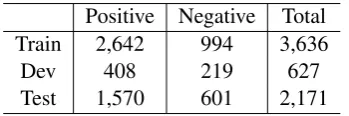
Table 5: Statistics of the SemEval 2013 Twitter sentiment classification dataset (positivevs nega-tive).

The statistics of our dataset crawled from Se-mEval 2013 are given in Table 5. The evalua-tion metric is the macro-F1 of sentiment classifi-cation. We train the joint model on the training set, tune parameters on the dev set and evaluate on the test set. We train the sentiment classifier with LibLinear (Fan et al., 2008) and utilize exist-ing sentiment lexicons 3 _{to extract}

classification-specific features. We randomly crawl 100M tweets from February 1st, 2013 to April 30th, 2013 with Twitter API, and use them to learn the phrase em-bedding with Skip-Gram 4_{. The vocabulary size}

of the phrase embedding is 926K, from unigram to 5-gram. The parameter -cin SVM is tuned on the dev-set in both baseline and our method. We run the L-BFGS for 50 iterations, and set the reg-ularization factorλas 0.003. The beam sizeN of the candidate generation model and the top-ranked segmentation numberKare tuned on the dev-set.

6.2 Baseline Methods

We compare the proposed joint model with the fol-lowing sentiment classification algorithms:

• DistSuper: We collect 10M balanced tweets

selected by positive and negative emoticons 5 _as

training data, and build classifier using the Lib-Linear and ngram features (Go et al., 2009; Zhao et al., 2012).

• SVM: The n-gram features and Support Vec-tor Machine are widely-used baseline methods to build sentiment classifiers (Pang et al., 2002). We use LibLinear to train the SVM classifier.

3_{In this work, we use HL (Hu and Liu, 2004),} M-PQA(Wilson et al., 2005),NRC Emotion Lexicon (Moham-mad and Turney, 2012), NRC Hashtag Lexiconand Senti-ment140Lexicon(Mohammad et al., 2013b).

4_{https://code.google.com/p/word2vec/}

5_{We use the emoticons selected by Hu et al. (2013). The}

positive emoticons are :) : ) :-) :D =), and the negative emoti-cons are :( : ( :-( .

• NBSVM: NBSVM (Wang and Manning,

2012) trades-off between Naive Bayes and NB-features enhanced SVM. We use NBSVM-bi be-cause it performs best on sentiment classification of reviews.

• RAE: Recursive Autoencoder (Socher et al., 2011) has been proven effective for sentiment clas-sification by learning sentence representation. We train the RAE using the pre-trained phrase embed-ding learned from 100M tweets.

• SentiStrength: Thelwall et al. (2012) build a

lexicon-based classifier which uses linguistic rules to detect the sentiment strength of tweets.

•SSWEu: Tang et al. (2014b) propose to learn

sentiment-specific word embedding (SSWE) from 10M tweets collected by emoticons. They apply SSWE as features for Twitter sentiment classifica-tion.

•NRC: NRC builds the state-of-the-art system in SemEval 2013 Twitter Sentiment Classifica-tion Track, incorporating diverse sentiment lexi-cons and hand-crafted features (Mohammad et al., 2013b). We re-implement this system because the codes are not publicly available. We do not di-rectly report their results in the evaluation task, as our training and development sets are smaller than their dataset. InNRC + PF, We concatenate the NRC features and the phrase embeddings fea-ture (PF), and build the sentiment classifier with LibLinear.

Except for DistSuper, other baseline method-s are conducted in a method-supervimethod-sed manner. We do not compare withRNTN(Socher et al., 2013b) be-cause the tweets in our dataset do not have accu-rately parsed results. Another reason is that, due to the differences between domains, the performance ofRNTN trained on movie reviews might be de-creased if directly applied on the tweets (Xiao et al., 2013).

6.3 Results and Analysis

Table 6 shows the macro-F1 of the baseline sys-tems as well as our joint model (JSC) on senti-ment classification of tweets (positivevsnegative).

cap-Method Macro-F1

DistSuper + unigram 61.74

DistSuper + 5-gram 63.92

SVM + unigram 74.50

SVM + 5-gram 74.97

Recursive Autoencoder 75.42

NBSVM 75.28

SentiStrength 73.23

SSWEu 84.98

NRC (Top System in SemEval 2013) 84.73

NRC + PF 84.75

JSC 85.51

Table 6: Macro-F1 for positivevsnegative classi-fication of tweets.

ture the semantic meaning of phrases. The integra-tion of high-order n-ngram (up to 5-gram) does not achieve significant improvement (+0.47%). The reason is that, if a sentence contains a bigram “not bad”, they will use “bad” and “not bad” as par-allel features, which confuses the sentiment clas-sification model. NBSVMandRecursive

Autoen-coder perform comparatively and have a big gap

in comparison with JSC. In RAE, the representa-tion of a sentence is composed from the represen-tation of words it contains. Accordingly, “great”

in “a great deal of” also contributes to the final

sentence representation via composition function.

JSC automatically conducts sentence segmenta-tion by considering the sentiment polarity of sen-tence, and utilize the phrasal information from the segmentations. Ideally, JSC regards phrases like

“not bad” and “a great deal of” as basic

compu-tational units, and yields better classification per-formance. JSC (85.51%) performs slightly better than the state-of-the-art systems (SSWEu, 84.98%;

NRC+PF, 84.75%), which verifies its

effective-ness.

6.4 Comparing Joint and Pipelined Models

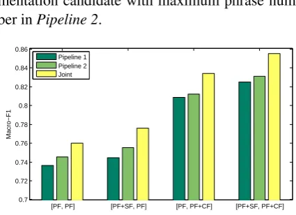
We compare the proposed joint model with pipelined methods on Twitter sentiment classifi-cation with different feature sets. Figure 2 gives the experiment results. The tick [A, B] on x-axis means the use of A as segmentation feature and the use of B as classification feature. PF

represents the phrase-embedding feature; SF and

CFstand for the segmentation-specific feature and classification-specific feature, respectively. We use the bag-of-word segmentation result to build sentiment classier inPipeline 1, and use the

seg-mentation candidate with maximum phrase num-ber inPipeline 2.

0.7 0.72 0.74 0.76 0.78 0.8 0.82 0.84 0.86

Macro−F1

[PF, PF] [PF+SF, PF] [PF, PF+CF] [PF+SF, PF+CF] Pipeline 1

Pipeline 2 Joint

Figure 2: Macro-F1 for positivevsnegative classi-fication of tweets with joint and pipelined models.

From Figure 2, we find that the joint model consistently outperforms pipelined baseline meth-ods in all feature settings. The reason is that the pipelined methods suffer from error propaga-tion, since the errors from linguistic-driven and bag-of-word segmentations cannot be corrected by the sentiment classification model. Besides, tra-ditional segmentors do not update the segmenta-tion model with the sentiment informasegmenta-tion of tex-t. Unlike pipelined methods, the joint model is capable to address these problems by optimizing the segmentation model with the classification re-sults in a joint framework, which yields better performance on sentiment classification. We also find that Pipeline 2always outperforms Pipeline 1, which indicates the usefulness of phrase-based segmentation for sentiment classification.

6.5 Effect of the beam sizeN

We investigate the influence of beam size N, which is the maximum number of segmentation candidates of a sentence. In this part, we clamp the feature set as [PF+SF, PF+CF], and vary the beam size N in [1,2,4,8,16,32,64]. The experiment re-sults of macro-F1 on the development set are il-lustrated in Figure 3 (a). The time cost of each training iteration is given in Figure 3 (b).

1 2 4 8 16 32 64 0.81

0.82 0.83 0.84 0.85 0.86

Beam Size

Macro−F1

(a) Macro-F1 score for senti-ment classification.

1 2 4 8 16 32 64 0

20 40 60 80 100 120

Beam Size

Runtime (Second)

(b) Time cost (seconds) of each training iteration.

Figure 3: Sentiment classification of tweets with different beam sizeN.

Figure 3 (b), we can find that the runtime of each training iteration increases with larger beam size. It is intuitive as the joint model with larger beam considers more segmentation results, which in-creases the training time of the segmentation mod-el. We set beam size as 16 after parameter learn-ing.

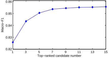
6.6 Effect of the top-ranked segmentation numberK

We investigate how the top-ranked segmentation number K affects the performance of sentimen-t classificasentimen-tion. In sentimen-this parsentimen-t, we sesentimen-t sentimen-the feasentimen-ture as [PF+SF, PF+CF], and the beam size as 16. The results of macro-F1 on the development set are il-lustrated in Figure 4.

1 3 5 7 9 11 13 15 0.82

0.83 0.84 0.85 0.86

Top−ranked candidate number

Macro−F1

Figure 4: Sentiment classification of tweets with different top-ranked segmentation numberK.

From Figure 4, we find that the classification performance increases with K being larger. The reason is that when a largerKis used, (1) at train-ing time, the sentiment classifier is built by ustrain-ing more phrasal information from multiple segmen-tations, which benefits from the ensembles; (2) at test time, the joint model considers several top-ranked segmentations and get the final sentiment polarity through voting. The performance remain-s remain-stable when K is larger than 7, as the phrasal information has been mostly covered.

7 Conclusion

In this paper, we develop a joint segmentation and classification framework (JSC) for sentiment analysis. Unlike existing sentiment classification algorithms that build sentiment classifier based on the segmentation results from bag-of-words or separate segmentors, the proposed joint model si-multaneously conducts sentence segmentation and sentiment classification. We introduce a marginal log-likelihood function to optimize the segmenta-tion model, and effectively train the joint mod-el from sentences annotated only with sentiment polarity, without segmentation annotations of sen-tences. The effectiveness of the joint model has been verified by applying it on the benchmark dataset of Twitter sentiment classification in Se-mEval 2013. Results show that, the joint model performs comparably with state-of-the-art meth-ods, and outperforms pipelined methods in various settings. In the future, we plan to apply the join-t model on ojoin-ther domains, such as movie/producjoin-t reviews.

Acknowledgements

We thank Nan Yang, Yajuan Duan, Yaming Sun and Meishan Zhang for their helpful dis-cussions. We thank the anonymous reviewers for their insightful comments and feedbacks on this work. This research was partly supported by National Natural Science Foundation of Chi-na (No.61133012, No.61273321, No.61300113). The contact author of this paper, according to the meaning given to this role by Harbin Institute of Technology, is Bing Qin.

References

Yoshua Bengio, Aaron Courville, and Pascal Vincent. 2013. Representation learning: A review and new

perspectives. IEEE Trans. Pattern Analysis and

Ma-chine Intelligence.

David M Blei, Andrew Y Ng, and Michael I Jordan. 2003. Latent dirichlet allocation. the Journal of ma-chine Learning research, 3:993–1022.

Yejin Choi and Claire Cardie. 2008. Learning with compositional semantics as structural inference for subsentential sentiment analysis. InProceedings of the Conference on Empirical Methods in Natural Language Processing, pages 793–801.

2011. Natural language processing (almost) from

scratch. Journal of Machine Learning Research,

12:2493–2537.

Xiaowen Ding, Bing Liu, and Philip S Yu. 2008. A holistic lexicon-based approach to opinion mining. In Proceedings of the International Conference on Web Search and Data Mining, pages 231–240. Li Dong, Furu Wei, Chuanqi Tan, Duyu Tang, Ming

Zhou, and Ke Xu. 2014. Adaptive recursive neural network for target-dependent twitter sentiment clas-sification. InProceedings of the 52nd Annual Meet-ing of the Association for Computational LMeet-inguistic- Linguistic-s, pages 49–54.

Rong-En Fan, Kai-Wei Chang, Cho-Jui Hsieh, Xiang-Rui Wang, and Chih-Jen Lin. 2008. Liblinear: A library for large linear classification. The Journal of Machine Learning Research, 9:1871–1874.

Ronen Feldman. 2013. Techniques and

application-s for application-sentiment analyapplication-siapplication-s. Communications of the

ACM, 56(4):82–89.

Kevin Gimpel, Nathan Schneider, Brendan O’Connor, Dipanjan Das, Daniel Mills, Jacob Eisenstein, Michael Heilman, Dani Yogatama, Jeffrey Flanigan, and Noah A. Smith. 2011. Part-of-speech tagging for twitter: Annotation, features, and experiments. InProceedings of the Annual Meeting of the Associ-ation for ComputAssoci-ational Linguistics, pages 42–47.

Xavier Glorot, Antoine Bordes, and Yoshua Bengio. 2011. Domain adaptation for large-scale sentiment

classification: A deep learning approach.

Proceed-ings of International Conference on Machine Learn-ing.

Alec Go, Richa Bhayani, and Lei Huang. 2009. Twit-ter sentiment classification using distant supervision.

CS224N Project Report, Stanford, pages 1–12. G.E. Hinton and R.R. Salakhutdinov. 2006.

Reduc-ing the dimensionality of data with neural networks.

Science, 313(5786):504–507.

Ming Hu and Bing Liu. 2004. Mining and summa-rizing customer reviews. InProceedings of the tenth ACM SIGKDD Conference on Knowledge Discovery and Data Mining, pages 168–177.

Xia Hu, Jiliang Tang, Huiji Gao, and Huan Liu. 2013. Unsupervised sentiment analysis with emo-tional signals. In Proceedings of the International World Wide Web Conference, pages 607–618.

Long Jiang, Mo Yu, Ming Zhou, Xiaohua Liu, and Tiejun Zhao. 2011. Target-dependent twitter

sen-timent classification. The Proceeding of Annual

Meeting of the Association for Computational Lin-guistics.

Nicola Jones. 2014. Computer science: The learning

machines. Nature, 505(7482):146.

Nal Kalchbrenner, Edward Grefenstette, and Phil Blun-som. 2014. A sentence model based on

convolu-tional neural networks. In Procedding of the 52th

Annual Meeting of Association for Computational Linguistics.

Hyun Duk Kim and ChengXiang Zhai. 2009. Gener-ating comparative summaries of contradictory

opin-ions in text. InProceedings of CIKM 2009. ACM.

Efthymios Kouloumpis, Theresa Wilson, and Johanna Moore. 2011. Twitter sentiment analysis: The good

the bad and the omg! In The International AAAI

Conference on Weblogs and Social Media.

Igor Labutov and Hod Lipson. 2013. Re-embedding

words. In Annual Meeting of the Association for

Computational Linguistics.

John Lafferty, Andrew McCallum, and Fernando Pereira. 2001. conditional random fields: Prob-abilistic models for segmenting and labeling

se-quence data. In Proceedings of international

con-ference on Machine learning. ACM.

Quoc Le and Tomas Mikolov. 2014. Distributed

repre-sentations of sentences and documents. Proceedings

of International Conference on Machine Learning. Dong C Liu and Jorge Nocedal. 1989. On the limited

memory bfgs method for large scale optimization.

Mathematical programming, 45(1-3):503–528. Bing Liu. 2012. Sentiment analysis and opinion

min-ing. Synthesis Lectures on Human Language Tech-nologies, 5(1):1–167.

Andrew L Maas, Raymond E Daly, Peter T Pham, Dan Huang, Andrew Y Ng, and Christopher Potts. 2011. Learning word vectors for sentiment analysis. In

Proceedings of the Annual Meeting of the Associ-ation for ComputAssoci-ational Linguistics.

Tomas Mikolov, Ilya Sutskever, Kai Chen, Greg Cor-rado, and Jeffrey Dean. 2013. Distributed represen-tations of words and phrases and their

composition-ality. Conference on Neural Information Processing

Systems.

Jeff Mitchell and Mirella Lapata. 2010. Composition in distributional models of semantics. Cognitive Sci-ence, 34(8):1388–1429.

Margaret Mitchell, Jacqui Aguilar, Theresa Wilson, and Benjamin Van Durme. 2013. Open domain

tar-geted sentiment. InProceedings of the 2013

Con-ference on Empirical Methods in Natural Language Processing, pages 1643–1654.

Saif M Mohammad and Peter D Turney. 2012.

Crowd-sourcing a word–emotion association lexicon.

Com-putational Intelligence.

Saif M Mohammad, Bonnie J Dorr, Graeme Hirst, and Peter D Turney. 2013a. Computing lexical contrast.

Saif M Mohammad, Svetlana Kiritchenko, and Xiao-dan Zhu. 2013b. Nrc-canada: Building the state-of-the-art in sentiment analysis of tweets. Proceedings of the International Workshop on Semantic Evalua-tion.

Tetsuji Nakagawa, Kentaro Inui, and Sadao Kurohashi. 2010. Dependency tree-based sentiment classifica-tion using crfs with hidden variables. InConference of the North American Chapter of the Association for Computational Linguistics, pages 786–794.

Alexander Pak and Patrick Paroubek. 2010. Twitter as a corpus for sentiment analysis and opinion mining. InProceedings of Language Resources and Evalua-tion Conference, volume 2010.

Georgios Paltoglou and Mike Thelwall. 2010. A s-tudy of information retrieval weighting schemes for

sentiment analysis. InProceedings of Annual

Meet-ing of the Association for Computational LMeet-inguistic- Linguistic-s, pages 1386–1395.

Bo Pang and Lillian Lee. 2008. Opinion mining and sentiment analysis. Foundations and trends in infor-mation retrieval, 2(1-2):1–135.

Bo Pang, Lillian Lee, and Shivakumar Vaithyanathan. 2002. Thumbs up?: sentiment classification using

machine learning techniques. InProceedings of the

Conference on Empirical Methods in Natural Lan-guage Processing, pages 79–86.

Yelong Shen, Xiaodong He, Jianfeng Gao, Li Deng, and Gr´egoire Mesnil. 2014. Learning semantic rep-resentations using convolutional neural networks for

web search. InProceedings of the companion

publi-cation of the 23rd international conference on World wide web companion, pages 373–374.

Richard Socher, J. Pennington, E.H. Huang, A.Y. Ng, and C.D. Manning. 2011. Semi-supervised recur-sive autoencoders for predicting sentiment

distribu-tions. InConference on Empirical Methods in

Nat-ural Language Processing, pages 151–161.

Richard Socher, Brody Huval, Christopher D. Man-ning, and Andrew Y. Ng. 2012. Semantic Com-positionality Through Recursive Matrix-Vector

S-paces. InProceedings of the Conference on

Empiri-cal Methods in Natural Language Processing.

Richard Socher, Danqi Chen, Christopher D Manning, and Andrew Y Ng. 2013a. Reasoning with neu-ral tensor networks for knowledge base completion.

The Conference on Neural Information Processing Systems.

Richard Socher, Alex Perelygin, Jean Wu, Jason Chuang, Christopher D. Manning, Andrew Ng, and Christopher Potts. 2013b. Recursive deep models for semantic compositionality over a sentiment

tree-bank. InConference on Empirical Methods in

Nat-ural Language Processing, pages 1631–1642.

Maite Taboada, Julian Brooke, Milan Tofiloski, Kim-berly Voll, and Manfred Stede. 2011.

Lexicon-based methods for sentiment analysis.

Computa-tional linguistics, 37(2):267–307.

Duyu Tang, Furu Wei, Bing Qin, Ming Zhou, and Ting Liu. 2014a. Building large-scale twitter-specific sentiment lexicon : A representation

learn-ing approach. In Proceedings of COLING 2014,

the 25th International Conference on Computation-al Linguistics, pages 172–182.

Duyu Tang, Furu Wei, Nan Yang, Ming Zhou, Ting Liu, and Bing Qin. 2014b. Learning sentiment-specific word embedding for twitter sentiment clas-sification. InProceedings of the 52nd Annual Meet-ing of the Association for Computational LMeet-inguistic- Linguistic-s, pages 1555–1565.

Mike Thelwall, Kevan Buckley, and Georgios Pal-toglou. 2012. Sentiment strength detection for the social web. Journal of the American Society for In-formation Science and Technology, 63(1):163–173. Peter D Turney. 2002. Thumbs up or thumbs down?:

semantic orientation applied to unsupervised classi-fication of reviews. InProceedings of Annual Meet-ing of the Association for Computational LMeet-inguistic- Linguistic-s, pages 417–424.

Sida Wang and Christopher D Manning. 2012. Base-lines and bigrams: Simple, good sentiment and topic

classification. InProceedings of the Annual

Meet-ing of the Association for Computational LMeet-inguistic- Linguistic-s, pages 90–94.

Theresa Wilson, Janyce Wiebe, and Paul Hoffmann. 2005. Recognizing contextual polarity in phrase-level sentiment analysis. InProceedings of the Con-ference on Empirical Methods in Natural Language Processing, pages 347–354.

Min Xiao, Feipeng Zhao, and Yuhong Guo. 2013. Learning latent word representations for domain adaptation using supervised word clustering. In Pro-ceedings of the 2013 Conference on Empirical Meth-ods in Natural Language Processing, pages 152– 162, October.

Ainur Yessenalina and Claire Cardie. 2011. Compo-sitional matrix-space models for sentiment analysis. InProceedings of Conference on Empirical Methods in Natural Language Processing, pages 172–182. Jiajun Zhang, Shujie Liu, Mu Li, Ming Zhou, and

Chengqing Zong. 2014. Bilingually-constrained

phrase embeddings for machine translation. In

Pro-ceedings of the 52nd Annual Meeting of the Associa-tion for ComputaAssocia-tional Linguistics, pages 111–121. Jichang Zhao, Li Dong, Junjie Wu, and Ke Xu. 2012.

Moodlens: an emoticon-based sentiment analysis

system for chinese tweets. In Proceedings of the