Online Full Text

(1)

Abstract—In this paper, finite element analysis of residual

thermal stresses in fiber-reinforced composites has been carried out. For a more realistic simulation of the microstructure of these materials subjected to different loadings, a representative volume element (RVE) may be used. In this paper, three different types of RVE configurations, circular, square and hexagonal are modeled and the effects of each type of fiber packing are studied. A mono fiber circular unit cell is considered using Finite Element (FE) method. Extending the mono fiber model, FE models with different arrays of fibers have been created to investigate the effects of neighboring fibers on the results. The results obtained are used to introduce new boundary conditions for the mono fiber model to make it able to predict the macro behavior in an efficient way. In all steps, the results are also compared with theoretical results presented in the literature. The boundary conditions presented in this research are proved to model the overall behavior efficiently.

Index Terms— fibrous composite material, finite element, representative volume element, inhomogeneous interphase, boundary conditions.

I. INTRODUCTION

Composite materials are becoming an essential part of present engineered materials because they offer advantages such as higher specific stiffness and strength, better fatigue strength and improved corrosion resistance compared to conventional materials. These high performance composites consist of different constituents. Subjected to thermal or thermo-mechanical loads, different deformations occur in different constituents leading to large differences of deformations and stresses between these constituents, which are known as residual deformations and stresses. However, the use of composite materials is limited by the lack of efficient tools to predict their degradation and lifetime under service loads, environment and the process induced residual stresses. For a more realistic simulation of the microstructure of these materials subjected to mechanical, thermal or

Manuscript received March 23, 2010.

M. M. Shokrieh is with Iran University of Science and Technology, Composite Research Laboratory, Center of Excellence in Solid Mechanics and Dynamics, Mechanical Engineering Department, Tehran, 16846-13114, Iran (corresponding author to provide phone: 00982177208127; fax:00982177240488; e-mail: shokrieh@ iust.ac.ir).

A. R. Ghanei Mohammadi is a graduate student in Iran University of Science and Technology Composite Research Laboratory, Center of Excellence in Solid Mechanics and Dynamics, Mechanical Engineering Department, Tehran, 16846-13114, Iran (e-mail: [email protected]).

[image:1.595.326.542.680.754.2]

thermo-mechanical loadings, a representative volume element (RVE) may be used. In the investigations applying FE method, one common procedure is the numerical generation of a RVE or a unit cell (UC) of the material being studied. A RVE or a UC is a statistical representation of the material [1]. Two major groups of these models are the composite cylinder models (CCM) [2] in which the RVE consist of two or more concentric cylinders and unit cell models (UCM) [3]-[5]. Because of its ability in reproducing the real stress and strain evolution, the simulation through a RVE may provide the understanding of the composite thermal behavior. This understanding is a need for the proposal of macroscopical results. In the analysis of the microstructure, the periodicity hypothesis of the fiber within the composite has been traditionally employed. This hypothesis reduces the analysis of the microstructure to the analysis of a single unit cell (the simpler RVE) and may lead to analytical solutions [6]. Three representative volume elements (Fig. 1) based on the 3-D elasticity theory have been proposed in (Liu and Chen, 2002) for the study of fiber reinforced composites. They are the cylindrical RVE (Fig. 1(a)), square RVE (Fig. 1(b)) and hexagonal RVE (Fig. 1(c)). The cylindrical RVE can be applied to model the models including different diameters (Hyer, 1998). Under axisymmetric as well as antisymmetric loading, a 2-D axisymmetric model can be applied for the cylindrical RVE, which can significantly reduce the computational work (Liu and Chen, 2002). The square RVE models can be applied when the conventional fiber-reinforced composites are arranged evenly in a square array, while the hexagonal RVE models can be applied when they are in a hexagonal array, in the transverse direction. These RVEs can be used to study the interactions with the matrix, such as the load transfer mechanism and stress distributions along the interfaces (Liu and Chen, 2002) or to evaluate the effective material properties of the composites [7].

Fig. 1 three representative volume elements [7]

Finite Element Modeling of Residual Thermal

Stresses in Fiber-Reinforced Composites Using

Different Representative Volume Elements

(2)

Although these unit cells can be useful for some purposes and can be employed successfully in two-scale methods to reproduce macroscopical behavior [8, 9], they do not reflect the reality of composite materials, in which the fiber is randomly distributed or it is placed among many other neighboring fibers, and consequently, they are not usable to simulate some of the complex mechanisms which take place in long fiber reinforced polymers and which may cause microscopic failure [10]. The selection of appropriate boundary conditions has been a challenge for many researchers. Since the RVEs must be modeled in a way that results obtained can efficiently describe the overall the composite material behavior, these boundary conditions have an important role in modeling the effect of the neighboring fibers, which are not considered in a mono fiber RVE cell. Many researchers have used micromechanical method to provide overall behavior of the composites from known properties of their constituents (fiber and matrix) through an analysis of a periodic representative volume element (RVE) or a unit-cell model [11,12]. In the macro-mechanical approach, on the other hand, the heterogeneous structure of the composite is replaced by a homogeneous medium with anisotropic properties. The advantage of the micromechanical approach is not only the global properties of the composites but also various mechanisms such as damage initiation and propagation, can be studied through the analysis [13, 14]. In the previous works, square and hexagonal arrays for RVEs have been studied extensively, but RVEs with curved boundaries, such as circular, have not been studied very much.

In this paper, a new unit cell finite element model has been presented to investigate fiber-reinforced composites subjected to thermal loading. An inhomogeneous interphase region has been assumed in the model. A mono fiber circular unit cell model is presented and then the model is generalized to include different geometrical configurations, such as a square unit cell, square cell arrays and hexagonal arrays. In order to present a mono fiber model which is efficiently able to model the macro thermal behavior of a fibrous composite material, the mono fiber model is extended and FE models with different arrays of fibers are created to investigate the effects of neighboring fibers on the results. The results obtained in these models are used to introduce new boundary conditions in the mono fiber model to make it able to predict the macro behavior in an efficient way. In all steps, the results are also compared with theoretical results available in the literature. The boundary conditions selected in the present work are proved to model the overall behavior of the mono fiber model efficiently.

II. FINITEELEMENTMODELING

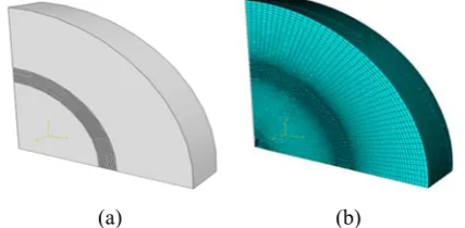
In this paper, a circular RVE, containing a fiber, interphase region and surrounding matrix, is presented and considered in the FE model. In order to reduce the FE problem size and the runtime, one fourth of the circular model is considered here. The interphase region is taken to be inhomogeneous. If the material properties of the interphase keep unchanged, the interphase is called homogeneous. Otherwise, it is called

considered in this research, the mechanical properties of this region undergo an exponential variation with the radial coordinate. The mathematical representation of this property variation can be written as [15]:

(

)

i f f i m

f r f

r

m

r r r r r r where t

t e r

e r t

t

f − = =

− − +

= −₋ ,

1 1

(1) where

)

,

(

E

L

E

T ₁₂ ₁₃ L T

t

=

ν

α

which it represents the transverse and longitudinal Young’s moduli ET and EL, Poisson’s ratios ν12 and ν13, and thermal expansion coefficients in the transverse and longitudinal directions αT and αL, respectively. Also, r is the radial distance from the fiber center and rf and ri are the fiber and interphase outer radii.

To apply the property variation above to the FE model, the interphase region is assumed to consist of some layers and the material properties are kept constant in each layer. To calculate the properties of each layer, a simple mathematical code is used to generate the properties as a function of the radial coordinate. The average value of two neighboring radial distances is calculated and taken to be the property value for the layer.

The Young’s moduli, Poisson’s ratios and thermal expansion coefficients of the fiber are taken to be ET=364.49 GPa, EL=488.45 GPa, ν12=0.2508, ν13=0.2, αT=6.25e-6/°C and αL=5.9e-6/°C. And those of the matrix are set to Em=200 GPa, νm=0.3, and αm=12.5e-6/°C. The outer radii of the fiber, interphase and matrix are taken as 5, 6 and 10 μm, respectively. The externally applied thermal load is a uniform temperature drop of -500 °C. ABAQUS 6.7-1 FE package has been used for modeling. Fig. 2 shows the circular mono fiber model used in this research.

(a) (b)

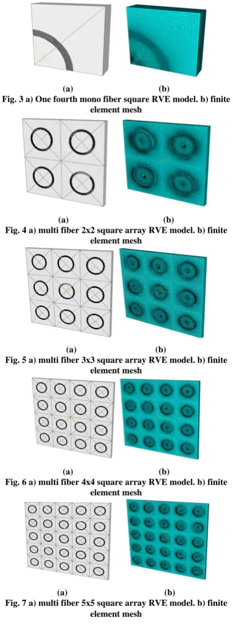
Fig. 2 a) One fourth mono fiber circular RVE model. b) finite element mesh

[image:2.595.321.535.499.604.2]

(3)

(a) (b)

Fig. 3 a) One fourth mono fiber square RVE model. b) finite element mesh

(a) (b)

Fig. 4 a) multi fiber 2x2 square array RVE model. b) finite element mesh

(a) (b)

As the third configuration possible, hexagonal packing of fibers in the matrix is modeled, too. Unlike the circular and square configuration, the simplest hexagonal RVE contains 2 fibers (see Fig.8). To investigate the effect of neighboring fibers and the convergence study of the results, an extended hexagonal unit cell (Fig.9) and a hexagonal array (Fig.10) are modeled.

(a) (b)

Fig. 8 a) hexagonal unit cell. b) finite element mesh

(a) (b)

Fig. 9 a) extended hexagonal unit cell. b) finite element mesh

(a) (b)

Fig. 10 a) hexagonal array. b) finite element mesh

These extended RVEs can help us have a better and more realistic understanding of overall macroscopic behavior of composites subjected to thermal loadings. The results of the extended models are compared with the results obtained from the mono fiber circular RVE to investigate the effect of neighboring fibers existence on its stress and displacement results and these results are used to select appropriate boundary conditions for the mono fiber model to make it able to predict the macro behavior of the fibrous composite material efficiently. Such a model can be used to represent all the fibers in the composite material.

Considering different theoretical models available [14,15] and based on a repetitive procedure, a new boundary condition is obtained and introduced in which generalized plane strain assumption (with a strain equal to 4.5624e-3) is made and also mechanical symmetry conditions are applied to the one fourth model of the circular RVE.

III. RESULTSANDDISCUSSION

The results of residual radial and circumferential and axial stresses and radial displacement around the interphase region are presented in this section.

COMPARISON OF RESULTS OF MONO FIBER CIRCULAR AND SQUARE AND HEXAGONAL

[image:3.595.51.287.51.683.2] [image:3.595.315.537.53.152.2] [image:3.595.318.537.179.278.2] [image:3.595.322.533.310.427.2]

(4)

circumferential and axial stresses and radial displacement around the interphase region are compared for the mono fiber square and circular and hexagonal models. (See Fig. 2,3 and 8)

radius (mm)

0.0045 0.0050 0.0055 0.0060 0.0065 0.0070

re

s

idu

al

r

a

di

al

s

tr

e

s

(

M

P

a)

-400 -350 -300 -250 -200 -150 -100

[image:4.595.328.521.57.208.2]

FE (square array model) FE (circular model) FE (hexagonal unit cell)

Fig. 11 Comparison of residual radial stresses for mono fiber square and circular and hexagonal models

radius (mm)

0.0045 0.0050 0.0055 0.0060 0.0065 0.0070

re

s

id

u

a

l

c

irc

u

m

fe

re

n

tia

l s

tre

s

(M

P

a

)

-400 -200 0 200 400 600

[image:4.595.58.278.122.253.2]

Fig. 12 Comparison of residual circumferential stresses for mono fiber square and circular and hexagonal models

radius (mm)

0.0045 0.0050 0.0055 0.0060 0.0065 0.0070

re

si

d

u

a

l a

x

ia

l st

re

ss

(

M

P

a

)

-1200 -1000 -800 -600 -400 -200 0 200 400 600

Fig. 13 Comparison of residual axial stresses for mono fiber square and circular and hexagonal models

radius (mm)

0.0045 0.0050 0.0055 0.0060 0.0065 0.0070

re

sid

ual r

a

d

ial disp

lacem

ent

(

m

)

-3.0e-5 -2.5e-5 -2.0e-5 -1.5e-5

[image:4.595.72.264.285.435.2]

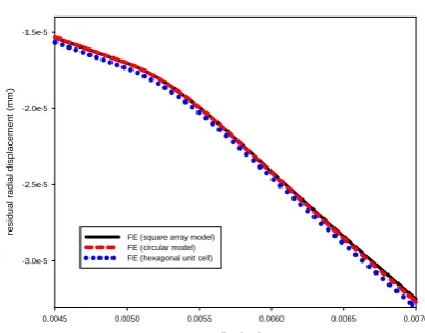
Fig. 14 Comparison of residual radial displacements for mono fiber square and circular and hexagonal models

As is shown, the results of residual axial stresses and radial displacements in all mono fiber models are quite similar. In the case of residual radial stresses, hexagonal unit cell shows less magnitude of these stresses and the residual radial stresses in square model are more than the other two models. In the interphase region, the results of hexagonal unit cell and the circular model are very close to each other. In the case of residual circumferential stresses in the fiber, the results of the square and hexagonal unit cell and in the matrix, the results of the circular and square models are very close. In all the regions, the circular model shows higher level of these stresses and in the interphase the results of all models are similar.

CONVERGENCE OF RESULTS FOR DIFFERENT FE ARRAYS

In Figs 15 to 22, the results of residual radial and circumferential and axial stresses and radial displacement around the interphase region are compared for the different square and hexagonal array FE models. (See Figs 4, 5, 6, 7, 9 and 10). As is shown, increasing the number of fibers in the model and creating a larger RVE, leads to more accurate results. Since the finite element mesh is chosen to be fine enough, the results converge very fast and increasing the number of fibers from 9 to 16 and 25 does not affect the results significantly.

radius (mm)

0.000 0.002 0.004 0.006 0.008 0.010 0.012

re

si

dual

radi

al

str

e

ss

(

M

Pa)

-400 -300 -200 -100 0 100

2x2 FE array 3x3 FE array 4x4 FE array 5x5 FE array

[image:4.595.66.269.481.624.2] [image:4.595.315.528.580.733.2]

(5)

radius (mm)

0.000 0.002 0.004 0.006 0.008 0.010

re

s

id

u

a

l

c

irc

u

m

fe

re

n

tia

l s

tre

s

(M

P

a

)

-400 -200 0 200 400 600

[image:5.595.318.533.54.216.2]

Fig. 16 Convergence of residual circumferential stresses for different square arrays

radius (mm)

0.000 0.002 0.004 0.006 0.008 0.010 0.012

re

si

du

a

l a

x

ia

l str

e

ss

(M

Pa

)

-1000 -800 -600 -400 -200 0 200 400

[image:5.595.62.269.64.217.2]

Fig. 17 Convergence of residual axial stresses for different square arrays

radius (mm)

0.0045 0.0050 0.0055 0.0060 0.0065 0.0070

resi

dual

radi

al

d

is

pl

acem

e

nt (

m

)

-3.0e-5 -2.5e-5 -2.0e-5 -1.5e-5

[image:5.595.317.533.317.593.2]

Fig. 18 Convergence of residual radial displacements for different square arrays

radius (mm)

0.0045 0.0050 0.0055 0.0060 0.0065 0.0070

re

sidu

al

ra

dia

l s

tress

(MP

a)

-400 -350 -300 -250 -200 -150 -100

FE (hexagonal unit cell) FE (extended hexagonal unit cell) FE (hexagonal array)

Fig. 19 Convergence of residual radial stresses for different hexagonal models

radius (mm)

0.0045 0.0050 0.0055 0.0060 0.0065 0.0070

res

idu

al

c

ircu

m

ferent

ia

l st

res

s

(MP

a)

-400 -200 0 200 400

Fig. 20 Convergence of residual circumferential stresses for different hexagonal models

radius (mm)

0.0045 0.0050 0.0055 0.0060 0.0065 0.0070

res

idual ax

ial st

ress (MP

a

)

-1000 -800 -600 -400 -200 0 200 400

Fig. 21 Convergence of residual axial stresses for different hexagonal models

radius (mm)

0.0045 0.0050 0.0055 0.0060 0.0065 0.0070

re

si

du

al

radi

al

di

spl

a

c

e

ment

(

mm)

-3.0e-5 -2.5e-5 -2.0e-5 -1.5e-5

Fig. 22 Convergence of residual radial displacements for different hexagonal models

COMPARISON OF RESULTS OF MONO AND MULTI FIBER FE MODELS AND A THEORETICAL MODEL

[image:5.595.62.275.426.573.2] [image:5.595.63.273.599.758.2]

(6)

radius (mm)

0.0045 0.0050 0.0055 0.0060 0.0065 0.0070

residua

l radial

st

ress (MPa)

-400 -350 -300 -250 -200 -150

You [15]

[image:6.595.63.277.58.204.2]

FE (mono fiber circular model) FE (5x5 multi fiber model) FE (hexagonal array)

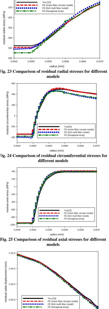
Fig. 23 Comparison of residual radial stresses for different models

radius (mm)

0.0045 0.0050 0.0055 0.0060 0.0065 0.0070

re

s

idua

l c

irc

um

fe

re

n

tia

l s

tr

e

ss

(

M

Pa)

-400 -200 0 200 400 600

You[15]

[image:6.595.59.278.59.375.2]

Fig. 24 Comparison of residual circumferential stresses for different models

radius (mm)

0.0045 0.0050 0.0055 0.0060 0.0065 0.0070

resid

ual axial stres

s (MPa)

-1000 -800 -600 -400 -200 0 200 400

You[15]

Fig. 25 Comparison of residual axial stresses for different models

radius (mm)

0.0045 0.0050 0.0055 0.0060 0.0065 0.0070

res

idu

al

r

adial

displacement (mm)

-3.0e-5 -2.5e-5 -2.0e-5 -1.5e-5

You [15]

Fig. 26 Comparison of residual radial displacements for different models

Following an extensive study, appropriate boundary conditions are selected for the mono fiber unit cell model and the results of the unit cell model show good agreement with You’s theoretical model [15]. As the next step, multi-fiber square arrays of fibers, such as 2x2, 3x3, 4x4 and 5x5 arrays and also extended hexagonal arrays are modeled using FEM. Comparing the results of the mentioned arrays, a convergence is observed in the results. Also, the results of array modeling are compared with the theoretical results and a good agreement is observed between the results in this part. These comparisons offered the chance to investigate the behavior of each possible configuration of RVEs and fiber packing and its effect on the residual stress and displacement distribution around the interface region of the fiber and matrix, incorporating an inhomogeneous interphase. The results show that each configuration gives slightly different results in different analyses and regions and one single model cannot be chosen as the most appropriate and it was shown that all these models do not have very much different behavior.

REFERENCES

[1] R. Hill, J. Mech. Phys. Solids 11 (1963) 357–372.

[2] Mikata Y, Taya M. 1985, “Stress field in a coated continuous fiber

composite subjected to thermo-mechanical loadings”. J Comp Mater; 19:554–78.

[3] J. Aboudi, “Micromechanical analysis of composites by the method of

cells”. Appl Mech Rev; 42: 1989, pp.193–221.

[4] RP. Nimmer “Fiber–matrix interface effects in the presence of

thermally induced residual stress”. J Comp Tech Res; 12: 1990, pp.65–75.

[5] D.D. Robertson, S. Mall “Micromechanical relations for

fiber-reinforced composites using the free transverse shear approach”. J Comp Tech Res; 15: 1993, pp.181–92.

[6] D. Trias, J. Costa, A. Turon and J. E. Hurtado, “Determination of the

critical size of a statistical representative volume element (SRVE) for carbon reinforced polymers”, Acta Materialia 54, 2006, pp.3471–3484.

[7] Y.J. Liu, X.L. Chen, “Evaluations of the effective material properties of

carbon nanotube-based composites using a nanoscale representative volume element”, Mechanics of Materials 35, 2003, pp.69–81

[8] E. Car, F. Zalamea, S. Oller, J. Miquel and E. On˜ate, “Numerical

simulation of composite materials: two procedures”. Inter J Solid Struct.; 39 (7), 2002, pp.1967–86.

[9] F. Feyel, “A multilevel finite element method (FE2) to describe the

response of highly non-linear structures using generalized continua”. Comput. Meth. Appl. Mech. Eng, 192, (28–30): 2003, pp.3233–44.

[10] T. Matsuda, N. Ohno, H. Tanaka andT. Shimizu, “Effects of fibre

distribution on elastic–viscoplastic behavior of long fibre-reinforced laminates”. Int. J. Mech. Sci. 45, 2003, pp.1583–98.

[11] J. Aboudi, “Mechanics of Composite Materials, A Unified

Micromechanical Approach”. Elsevier Science Publishers, Amsterdam, 1991.

[12] S. Nemat-Nasser , M. Hori,. “Micromechanics: Overall Properties of

Heterogeneous Materials”. Elsevier Science Publishers, Amsterdam, 1993.

[13] Z. Xia, Y. Chen and F. Ellyin, “A meso/micro-mechanical model for

damage progression in glass–fiber/epoxy cross-ply laminates by finite-element analysis”. Composite Science and Technology, 60, 2000, pp. 1171–1179.

[14] F. Ellyin, Z. Xia and Y. Chen,. “Viscoelastic micromechanical

modeling of free edge and time effects in glass fiber/epoxy cross-ply laminates”. Composites, Part A, 33, 2002, pp.399-409.

[15] L.H. You and X.Y. You, “A unified numerical approach for thermal

[image:6.595.58.285.66.706.2]