Online Full Text

(1)

Abstract - This work investigates the impact of the load

representation upon a power system security assessment. This is done according to two important aspects: the adopted direction for the load increment and the dynamic models used to represent its behavior. The first aspect is tackled through an evaluation of contingencies, which is based on the system’s load flow model for two load increment directions: the “traditional” approach, where the system active and reactive load demands are increased proportionally to the base case, and a second approach that regards the “worst case”, in which it is adopted the direction that gives the smallest “local” loading margin for the base case. The second aspect is tackled through a system multi-machine modelling that takes into account the impact of the generators, loads, Automatic Voltage Regulators (AVRs), Over Excitation Limiters (OXLs) and Load Tap Changers (LTCs) dynamic behavior. The dynamic responses of the system are compared to the most critical contingencies previously obtained. Some discrepancies existing in the power system security analysis are analysed for both the increment directions and the dynamic load models through simulations obtained for the IEEE 14 bus system.

Index Terms— Voltage stability, Load models, Power system

security, Power system dynamic simulation.

I. INTRODUCTION

Presently, power systems are facing a restructuring process due mainly to economical and environmental factors. From the economical viewpoint, the new reality imposed to power systems is characterized by a competitive atmosphere, among other factors, originated by the disintegration of the generating capacity. From the environmental viewpoint, the natural resources needed to expand those systems are becoming shorter than some years ago. Moreover, there are social pressures to preserve these resources and so minimise the environmental implications.

As a consequence, the possibility to attend new demand by expanding the power systems (installation of new generating units and transmission lines) is becoming highly jeopardized. Besides, transmission and generation reserves should be lesser than ever in order to minimise production and transmission

Manuscript received March 22, 2007.

José Geraldo B. M. de Andrade is with the Electrical Engineering Department, Polytechnic School of the University of São Paulo, Brazil ([email protected]).

Hernán Prieto Schmidt is with the Electrical Engineering Department, Polytechnic School of the University of São Paulo, Brazil ([email protected]).

costs, guaranteeing the competitiveness among companies and saving the already scarce natural resources. These facts make power systems operate with more reduced stability margins.

So, it is necessary to know the power systems operation limits in order to guarantee quality and safety margins to power system supplying. Among the limits commonly investigated (such as thermal overload limits and angular instability) voltage instability limit is seen as one of the prominent threats to the safe operation of the electric system [1]-[3]. This is the reason why in the last years there have been issued researches [4] on this topic. Moreover, it is known that the dynamic behavior of the load is the key element for a number of incidents related to voltage instability (and collapse) phenomenon observed [3].

This work investigates the impact of some aspects related to the load representation for the voltage stability assessment. From the static viewpoint, it is analysed the impact of adopting different directions for the load increment to the contingency screening and ranking process. From the dynamic viewpoint, it is analysed the impact of adopting different dynamic models to represent the load through a multimachine representation.

II. GENERIC REPRESENTATION OF THE POWER SYSTEM In a generic representation of the power system, the electric network is commonly represented through algebraic equations. On the other hand, short-term dynamics associated to generators, automatic voltage regulators (AVRs), turbines and induction motors are represented through differential equations. A combination of differential and discreet equations varying with time is used to analyse long-term dynamics associated to transformers load tap-changers (LTCs), over-excitation limiters (OXLs) of generators and power recovery characteristic of loads. The non-linear differential-algebraic equations (DAE) can be represented by the following equations [2]:

) , , , (

0=g x y zc zd ₍₁₎

) , , ,

(x y zc zd

f

x&= (2)

) , , ,

( c d

c

c h x y z z

z = (3)

)) ( , , , ( ) 1

(k h x y z z k

zd + = d c d (4)

Where,

y is the voltage vector in the buses.

x is the state variables vector associated to the short-term

dynamics.

A Contribution to the Voltage Stability Studies

within Power Systems: Some Aspects Related to

the Load Representation

(2)

zc and zd represent the continuous and discreet vectors,

respectively; associated to the long-term dynamics.

So, the mathematical model described by (1) through (4) regards the short and long-term dynamics simultaneously. It is known that the time constants characterizing the short and long-term dynamics in a power system can vary from microseconds to minutes, providing a stiff characteristic to the DAE [2] which hampers its numeric solution. This difficulty can be tackled using implicit integration methods having

A-stability properties and also variable-step integration strategies [5].

III. POWER SYSTEM SECURITY ANALYSIS

There is not yet full agreement on whether voltage stability should be evaluated through a static or a dynamic approach. The former uses a purely algebraic model that describes the power system behavior through (1); its solution is obtained similarly to the approach used to solve load flow. The latter alternative uses the generic model represented in (1)-(4) and requires a relatively bigger computational effort. It also needs an additional engineering work for analyzing the results [3].

So, the power system security analysis is usually accomplished using a combination of the two approaches previously mentioned. The static approach is used to filter the most critical contingencies that can take the system to a voltage instability condition or even to a voltage collapse. The dynamic approach is used to perform a detailed analysis of the most critical contingencies captured by the static approach. Its aim is to identify the actions that need to be adopted in order to improve the system security. The numeric methods used in the screening and ranking of the most critical contingencies as well as in the power system stability dynamic analysis are presented next.

IV. EVALUATION OF THE MOST CRITICAL CONTINGENCIES In order to select and classify the most critical contingencies, we adopt the post-contingency loading margin as severity index (SI). Such an index is calculated from a continuation power flow [6] along to a load increment direction. Next, a brief description of the continuation power flow method and an analysis on the load increment direction impact upon the system’s load margin calculation is presented.

A. Continuation Power Flow [6], [7]

The continuation power flow is based on the system static model (1). It basically calculates the successive equilibrium points for (5) assuming slow variations of the λ parameter which represents the increment in load demand and power supplied by the system generators.

) , (

0=g y λ (5)

Equation (5) can be re-written as load flow expressions:

) sin cos

( )

( ij ij ij ij

i j

j i Li

Gi P V V G B

P λ − λ =

∑

⋅ ⋅ ⋅ θ + ⋅ θ

∈

(6)

) cos sin

( )

( ij ij ij ij

i j

j i Li

Gi Q V V G B

Q λ − λ =

∑

⋅ ⋅ ⋅ θ − ⋅ θ

∈

(7)

The increments of the generators active power (8) and the demand in the buses (9) and (10) are given by:

) 1

( )

( Gi0 Gi

Gi P K

P λ = ⋅ +λ⋅ (8)

) 1

( )

( Li0 PLi

Li P K

P λ = ⋅ +λ⋅ (9)

) 1

( )

( Li0 QLi

Li Q K

Q λ = ⋅ +λ⋅ (10)

Where,

PLi0andQLi0 represent the load active and reactive power of the

ithbus, assuming the base case (λ=0).

PGi0is the active power supplied by the generator of the ithbus,

assuming the base case (λ=0).

KPLiandKQLiare coefficients defining the load power factor of

the ithbus.

KGiis a coefficient defining the generator’s participation factor

in the ithbus for a certain loading level (λ).

Equations (6)-(7) can be written in a compact form as: 0

) ( ) ,

(y =G y + ⋅d =

g λ λ (11)

In (11), d represents a vector indicating the direction of the

active and reactive power increment consumed by the loads and the active power supplied by the generators.

The successive solutions of (5), for different values of the λ

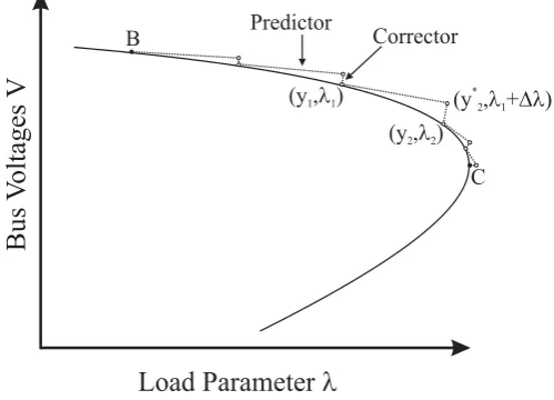
parameter, are obtained by the continuation power flow through a predictor-corrector scheme showed in Figure 1.

The predicting stage consists in obtaining, from a given point (y1, λ1), an approximate solution (y*2, λ1+Δλ) for the new

loading level λ2. In this work, the tangent vector (12) to the Vλ

curve is being used in the predicting stage. The correcting stage consists in calculating the (y2, λ2) point defined by the

intersection of the line perpendicular to the tangent vector passing through the (y*

2, λ1+Δλ) point and intersects the Vλ

[image:2.595.303.553.557.737.2]

curve. Such point is obtained using (13) and (14).

(3)

) , ( 1 ) , ( ) , ( 1 1 1 1 1 1 λ λ λ λ λ y y y g y g y ∂ ∂ ⋅ ⎟ ⎟ ⎠ ⎞ ⎜ ⎜ ⎝ ⎛ ∂ ∂ − = ∂

∂ − (12)

) , (

0=g y λ (13)

) (

0 1 1 1 y1 y y1 y1

T _⋅ ₋ ₋_Δ

Δ + Δ − − ⋅ Δ

= λ λ λ λ (14)

By applying the described methodology, the loading margin

λC-λB, seen in Figure 1, is obtained for each analysed

contingency.

B. Evaluation of the Load Increment Direction

In order to evaluate the impact of the adopted direction for the load increment (evaluation of the system security), it is considered two directions of load increment: one direction, herein referred to as “traditional”, where the active and reactive demands increase proportionally to the base case (KPLi=KQLi=1

in (9) and (10)) and another direction, referred to as “worst case” [8]. In the “worst-case”, the adopted direction for the active and reactive load increment corresponds to the smallest local loading margin for the case base.

The d* direction corresponding to the “worst case” is obtained

using the methodology proposed in [8] and [9], briefly described next:

(i). Select any vector di = d0 as an initial estimation for the

d* direction corresponding to the “worst case” of load

increment, |d0|=1;

(ii). Stress the system by incrementing λ according to the di

direction until the Jacobian matrix of the load flow turns singular (see point C in Fig.1);

(iii). Make di+1 = wi.∂g(y, λ)/∂λ, |di+1|=1;

(iv). Repeat steps (ii), (iii) and (iv) until di converges for

the value of d*.

Where,

wiis the left eigenvector with respect to the load flow

Jacobian ∂g(y, λ)/∂ y.

Once applied the two methodologies described in Sections IV(A) and IV(B), it is possible to obtain a list of the most severe contingencies for the two load increment directions previously considered. Next, the most severe contingencies for both scenarios are analysed using a multi-machine simulator.

V. VOLTAGE STABILITY DYNAMIC ANALYSIS

In order to investigate the load dynamic behavior for the most critical contingencies, we developed a multi-machine dynamic simulator based on the network’s generic model described in (1)-(4). This simulator is based on the DASSL (Differential Algebraic System SoLver) solver [10] which is adequate for the solution of stiff differential-algebraic equations. Next, a description of the DASSL method and the dynamic models of the devices included in such a simulator are presented.

A. The DASSL Solver [10]

The DASSL solver is suited to solve stiff

differential-algebraic equations having indexes zero and one, such as: ⎩ ⎨ ⎧ = = = ) , ( 0 ) , ( ) , , ( t y g t y f y y y t

F & & (15)

0 0) (t y

y = (16)

0 0) (t y

y& = & (17)

Where,

F(t, y, dy/dt) represents the system described in (1)-(4). y and dy/dt are vectors of order N having the variables described in Section II.

DASSL is a variable step and variable order DAE solver based on the BDF methods (Backward Differentiation Formulae). It presents two steps for solving (15).

In the predictor step it uses a divided difference polynomial (18) in order to interpolate the yj+1-k solution points of the last k

time intervals and so obtaining the first approximation of yj+1.

k j j k j j j j j j j j y y t t t t t t y y t t y t y − + − − − + ⋅ − ⋅ − ⋅ − + + ⋅ − + = , , ) ( ) ( ) ( , ) ( ) ( 1 1 1 1 K

K ₍₁₈₎

Where the divided differences are defined by:

j

j y

y = (18)

k j j k j j j k j j j k j j t t y y y y y y y y − − − − + − − − ₋ − = , , , , , , ,

,K 1K 1 1 2 K (19)

In the corrector step the dy/dt derivative (15) is estimated using a BDF polynomial (20) with order k, obtaining the non-linear algebraic equations (21).

∑

= +− + + ⋅ ⋅ = ⋅ k r j j r j

r y h F y t

0

1 1 0

1 β ( , ,)

α (20)

Where,

αr and β0 represent the coefficients that depend on the k order

selected for the BDF formulae.

h is the length of the jth_{integration step.}

⎪⎩ ⎪ ⎨ ⎧ = = ⋅ ⋅ − ⋅ + = + + = +− + + + + + +

∑

0 ) , ( 0 ) , ( ) , , ( 1 1 0 1 1 0 1 1 1 1 1 j j k r j j r j r j j j j t y g t y f h y y y y t

F & α β (21)

Equation (21) can be solved using a modified Newton method [10].

The method’s order and step selection is based on the local truncation error control. At the end of each integration step h it is verified if the estimative for the local truncation error is within the allowed tolerance. Should it be the case the step is accepted and it is determined, using the same error, if there is margin to increase the integration step. Conversely, the step is rejected and it is determined the length of the necessary step so that the error remains within the allowed tolerance [10].

B. Device Models Included in the Dynamic Simulator

(4)

Generators: It is considered only the IEEE 1.1 model, as recommended by [11] for stability studies, neglecting the saturation effect.

(

)

(

)

0

1 ' ' '

0

' ₋ _⋅ ₋ ₋ ₋ _⋅ ₌

d d d q fd d

q T E E x x i

E& (22)

(

)

(

)

0

1 ' ' '

0

' ₋ _⋅ ₋ ₊ ₋ _⋅ ₌

q q q q q

d T E x x i

E& (23)

0

'

' ₊ _⋅ ₊ _⋅ ₌

− q a q d d q E r i x i

E (24)

0

'

' ₊ _⋅ ₋ _⋅ ₌

− d a q q q d E r i x i

E (25)

(

)

(

ω ω

)

ω

ω 0

' ' ' ' 0

2⋅ ⋅ − ⋅ − ⋅ − − ⋅ ⋅ − ⋅

= T E i E i x x i i D

H m q q d d q d q d

& (26)

0 = −ω

δ& (27)

Where,

E’d and E’q are, respectively, the direct and quadrature axis

transient voltages (in per unit).

Ed and Eq are, respectively, the direct and quadrature axis

voltages (in per unit).

Efd is the field voltage in per unit.

id, iq are, respectively, the direct and quadrature axis currents

(in per unit).

T’d0 and T’q0 are, respectively, the direct and quadrature axis

open-circuit transient time constants (in seconds).

ra, xd and xq are, respectively, the armature resistance and the

direct and quadrature axis synchronous reactances (in per unit).

x’d and x’q are, respectively, the direct and quadrature axis

transient reactances (in per unit).

Tm and D are, respectively, the mechanic torque and the

damping coefficient (in per unit).

w, w0 and δ, respectively, are the rotor angular frequency (in

radians/s), the synchronous reference frame angular frequency (in radians/s) and the load angle (in radians).

AVRs: It considers a Proportional-Integer (PI) type controller, as described in (28), with the output Efd constrained in a range

from EMIN to EMAX due to the presence of an anti-windup limiter

[12].

(

)

1 0

' ₋ _⋅ ₋ ₋ ₊ _⋅ ₌

fd A OXL G ref A A

fd K T V V V T E

E& (28)

Where,

KA and TA are, respectively, the AVR gain (in per unit) and the

time constant (in seconds).

Vref, VOXL and VGare, respectively, the AVR reference voltage,

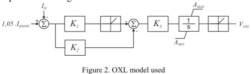
[image:4.595.44.296.635.710.2]

the OXL output and the generator bus voltage (in per unit). OXLs: It considers the model suggested in [3] and which is represented in Figure 2.

Figure 2. OXL model used Where,

K1, K2 and K3 are settings that determine the OXL inverse time

characteristic (in per unit).

Ifd and IfdNOM are, respectively, the generator field current and

the AVR field current setting, respectively. (in per unit).

VOXL is OXL output signal (in per unit). It’s constrained in a

range from AMIN to AMAX due to the presence of an anti-windup

limiter [12].

LTCs: It considers the continuous model suggested by [2] and described in (29).

(

−

)

=0

−V Vref TC

r& (29)

Where,

V and Vref are, respectively, the LTC controlled voltage and

reference voltage setting (in per unit).

TC is the time constant (in seconds).

r is the tap value (in per unit/per unit). It’s constrained in a range from rMIN to rMAX due to the presence of an anti-windup

limiter [12].

Loads: Aside of the static ZIP and exponential load models, it is considered the dynamic models proposed by Hill et al [13] and Ihara et al [14].

Hill et al model [13]

(

_V _V

)

S _P

(

_V _V

)

T

P P P

TP r r

α α

0 0 0

0⋅ − ⋅

= +

⋅& (30)

(

_V _V

)

S _Q

(

_V _V

)

T

Q Q Q

TQ r r

β β

0 0 0

0⋅ − ⋅

= +

⋅ & (31)

(

_V _V

)

T

P P

P r

α

0 0⋅

+

= (32)

(

_V _V

)

T

Q Q

Q r

β

0 0⋅

+

= (33)

Where,

V and V0 are, respectively, the post and pre-contingency load

voltages (in per unit).

P, P0 e Pr are, respectively, the total, pre and post-contingency

active powers (in per unit).

Q, Q0 e Qr are, respectively, the total, pre and post-contingency

reactive powers (in per unit).

TP and TQare the recovery time constants (in seconds).

αS andβSare, respectively, the active and reactive steady-state

voltage dependencies (in per unit/per unit).

αT and βT are, respectively, the active and reactive transient

voltage dependencies(in per unit/per unit). Ihara et al model [14]:

(

)

{

₁ _K _V ₁

}

(

₁ _P

)

_P

(

_G ₁

)

_V2

P= + P⋅ − ⋅ − drop + dyn⋅ − ⋅ (34)

(

)

{

₁ _K _V ₁

} (

₁ _Q

)

_Q

(

_B ₁

)

_V2

Q= + Q⋅ − ⋅ − drop + dyn⋅ − ⋅ (35)

(

1

)

_⋅

(

_⋅ 2₋1

)

−

= T G V

G& P (36)

( )

1 _⋅

(

_⋅ 2₋1

)

−

= T B V

B& Q (37)

Where,

V, P and Q are, respectively, the voltage and the active and reactive powers (in per unit).

KP and KQ are, respectively, the active and reactive voltage

dependencies (in per unit/per unit).

TP and TQ are, respectively, the recovery time constants (in

seconds).

G, Pdrop and Pdyn are, respectively, the load conductance (in per

(5)

under-voltage protection) and the percent of dynamic active load.

B, Qdrop and Qdyn are, respectively, the load susceptance (in per

unit), the percent of disconnected reactive load (due the under-voltage protection) and the percent of dynamic reactive load.

VI. NUMERICAL RESULTS

The methodologies, described in Sections IV and V, have been examined on the IEEE 14-bus system, which static and dynamic data were obtained, respectively, from [15] and [16].

Figure 3 shows a comparison between the “traditional” and the “worst-case” load increment directions. It can be seen that by incrementing the system load along the “traditional” direction the generators can supply an additional of 112.98 MW. By using the “worst case” it reduces to 75.90 MW. Similarly, Figure 4 shows that these additional reactive power supplies are bounded in, respectively, 118.36 MVAr using the “traditional” direction and 78.46 MVAr using the “worst case” direction.

0 20 40 60 80 100 120 140 160

P1 P2 P3 P4 P5 P6 P7 P8 P9 P10 P11 P12 P13 P14

[image:5.595.309.547.114.338.2]

P_base-case[MW] PMAX_worst-case [MW] PMAX_traditional [MW] Figure 3. Active load margins in the IEEE 14-bus system along

“traditional” and “worst-case” increment directions

-15 -5 5 15 25 35 45 55

Q1 Q2 Q3 Q4 Q5 Q6 Q7 Q8 Q9 Q10 Q11 Q12 Q13 Q14

[image:5.595.52.287.322.413.2]

Q_base-case[MVAr QMAX_worst-case [MVAr] QMAX_traditional [MVAr] Figure 4. Reactive load margins in the IEEE 14-bus system along

Table 1 shows the results obtained for the contingency analysis applied to the IEEE 14-bus system using the methodology presented in Section IV(A) and the UWPFLOW program [7]. It can be seen that four out of the five contingencies classified as the severest, are captured by the contingency ranking module. This occurs for the two load increment directions analysed. Additionally, it can be observed that the six contingencies classified as severest for the “worst-case” direction present values of severity index less than the one of the severest contingency captured in the “traditional” direction. This result shows the strong dependency between the adopted load increment direction and the contingency screening and ranking for voltage security assessment.

TABLE 1.CONTINGENCY RANKING FOR THE (A) TRADITIONAL AND (B)

WORST-CASE DIRECTIONS (IEEE14-BUS SYSTEM)

“Traditional” direction

Contingency SI

1 T05_06 0.19488

2 L02_03 0.23615

3 L01_05 0.27734

4 L07_09 0.29764

5 T04_07 0.37272 6 L01_02 0.37704 7 L02_04 0.3989 8 L09_14 0.41708 9 L04_05 0.42282 10 L06_13 0.42529 11 T04_09 0.43266 12 L02_05 0.43565 13 L09_10 0.46697 14 L13_14 0.47818 15 L06_11 0.47847 16 L06_12 0.48564 17 L12_13 0.49196 18 L03_04 0.49489 19 L10_11 0.49517

“Worst-case” direction

Contingency SI

1 T05_06 0.08376

2 L01_05 0.15538

3 L07_09 0.15872

4 L09_14 0.18402

5 L02_03 0.18694

6 T04_07 0.19413 7 L06_13 0.20895 8 L02_04 0.21213 9 L09_10 0.21439 10 L01_02 0.21673 11 L02_05 0.22497 12 T04_09 0.22708 13 L06_12 0.23825 14 L04_05 0.24339 15 L03_04 0.25072 16 L06_11 0.25213 17 L13_14 0.25589 18 L10_11 0.26161 19 L12_13 0.26258

In order to investigate the impact of load increment direction on load recovery mechanism we perform simulations of some contingencies in the IEEE 14 bus system using the dynamic load model proposed in [13] in buses 13 and 14. Table 2 shows the parameters used in load buses 13 and 14.

TABLE 2.PARAMETERS USED IN THE LOAD MODELS OF

BUSES 13 AND 14(IEEE14-BUS SYSTEM)

Bus αS αT βS βT TP [s] TQ [s]

13 -0.32 1.65 -0.48 2.22 70 78 14 -0.16 1.31 -0.77 2.08 61 88 Figures 5 and 6 shows, respectively, the time evolution of bus 13 voltage, load active and reactive power consumption during the contingency L06_13 for a load consumption increment of 30% above the base case along the “traditional” and the “worst-case” directions.

0.8 0.85 0.9 0.95 1 1.05 1.1

0 100 200 300 400 500 600

time [s]

Bu

s V

ol

ta

g

[image:5.595.53.284.454.547.2] [image:5.595.313.554.569.693.2]

(6)

0.1 0.12 0.14 0.16 0.18 0.2 0.22 0.24 0.26

0 100 200 300 400 500 600

time [s]

PL

oa

d

[image:6.595.55.292.89.223.2]

P_Bus13[pu] (base) P_Bus13[pu] (traditional) P_Bus13[pu] (worst)

Figure 6. Load recovery (active power) at Bus 3 for “base case”, “traditional” and “worst-case” increment directions

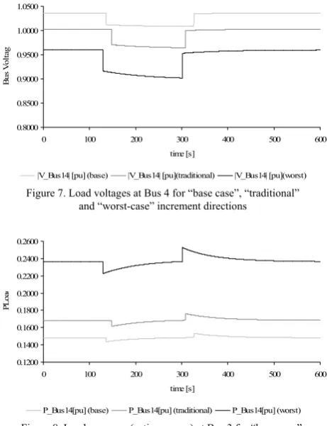
Similarly, Figs 7 and 8 shows, respectively, the time evolution of bus 14 voltage, load active and reactive power consumption during the contingency L06_13 for a load consumption increment of 30% above the base case along the “traditional” and the “worst-case” directions.

0.8000 0.8500 0.9000 0.9500 1.0000 1.0500

0 100 200 300 400 500 600

time [s]

B

us

V

olta

g

and “worst-case” increment directions

0.1200 0.1400 0.1600 0.1800 0.2000 0.2200 0.2400 0.2600

0 100 200 300 400 500 600

time [s]

PL

oa

d

[image:6.595.53.284.333.634.2]

P_Bus14[pu] (base) P_Bus14[pu] (traditional) P_Bus14[pu] (worst) Figure 8. Load recovery (active power) at Bus 3 for “base case”,

Figures 5 and 7 shows the large differences among voltage time evolution of buses 13 and 14 only by varying the load increment direction used in voltage stability dynamic analysis. Cleary, for both buses, the “worst-case” direction is the severest among the three adopted directions.

Figures 6 and 8 shows the time evolution of load buses 13 and 14 active power responses. Cleary the load active power recovery is more severe in the “worst-case” direction.

VII. CONCLUSIONS AND FUTURE WORK

We have examined the impact of load representation upon a power system security assessment. Two important aspects are investigated: the adopted direction for load increment and the dynamic load models used to represent its behavior. These two aspects are evaluated by using: a method to determine the “traditional” and “worst-case” load increment directions [8], [9]; a continuation power flow algorithm [7] for contingency screening and ranking; and a DASSL [10] based power system simulator to perform the dynamic analysis of the most critical contingencies. The results obtained for the IEEE 14 bus system show the high impact of the analysed aspects in power system security assessment.

A similar investigation for the Ihara[14] dynamic load model and an extension of this work for the IEEE 30 and 57-bus systems are currently underway.

REFERENCES

[1] Cutsem, T. V. Voltage instability: phenomena, countermeasures, and analysis methods. Proceedings of the IEEE, v. 88, n. 2, p. 208–227, Feb. 2000.

[2] Cutsem, T. V.; Vournas, C. Voltage stability analysis of electric power systems. Kluwer Academic Publishers, 1998. 396 p.

[3] Taylor, W. C. Power System Voltage Stability. McGraw-Hill Education, 1994. 272 p.

[4] Ajjarapu, V.; and Lee, B. Bibliography on voltage stability, IEEE Trans. on Power Systems, vol. PWRS-13, pp. 115–125, February 1998. [5] Astic, J. Y.; Bihain, A.; Jerosolimski, M. The mixed Adams - BDF

Variable Step Size Algorithm to Simulate Transient and Long Term Phenomena In Power Systems, IEEE Trans. on PS, Vol. 9, No. 2, May 1994.

[6] Ajjarapu, V.; Christy, C. The continuation power flow: a tool for steady state voltage stability analysis. Power Systems, IEEE Transactions on, v. 7, n. 1, p. 416–423, Feb. 1992.

[7] Canizares, C. A.; Alvarado, F. L. ‘UWPFLOW software: continuation and direct methods to locate fold bifurcations in AC/DC power systems’. Available: http://www.power.uwaterloo.ca/~claudio/software

[8] Dobson, I.; Lu, L. New methods for computing a closest saddle node bifurcation and worst case load power margin for voltage collapse Power Systems, IEEE Transactions on, 1993, 8, 905-913.

[9] Dobson, I. An iterative method to compute a closest saddle node or Hopf bifurcation instability in multidimensional parameter space Circuits and Systems, 1992. ISCAS '92. Proceedings, 1992 IEEE International Symposium on, 1992, 5, 2513-2516, vol.5.

[10] Ascher, U.M., Petzold, L.R. Computer methods for ordinary differential equations and differential-algebraic equations SIAM: Society for Industrial and Applied Mathematics, 1998, 332.

[11] Dandeno P. L. et al. IEEE Guide for synchronous generator modeling practices in stability analyses, IEEE Std. 1110-1991.

[12] Smith, C. A.; Corripio, A. B. Principles and Practice of Automatic Process Control. John Wiley & Sons, 1997.

[13] Hill, D.; Nonlinear dynamic load models with recovery for voltage stability studies Power Systems, IEEE Transactions on, 1993, 8, 166-176. [14] Ihara, S.; Tani, M, Tomiyama, K. Residential load characteristics

observed at KEPCO power system Power Systems, IEEE Transactions on, 1994, 9, 1092-1101.

[15] Power Systems Test Case Archive – UWEE. Available:

www.ee.washington.edu/research/pstca/