Self localization of PIRATE inside a partially structured environment

Full text

(1)University of Twente EEMCS / Electrical Engineering Control Engineering. Self Localization of PIRATE Inside a Partially Structured Environment. Twan Mennink MSc report. Supervisors: prof.dr.ir. S. Stramigioli dr. R. Carloni ir. E.C. Dertien dr. C.J.A. Pulles December 2010 Report nr. 027CE2010 Control Engineering EE-Math-CS University of Twente P.O.Box 217 7500 AE Enschede The Netherlands.

(2) ii. Self Localization of PIRATE Inside a Partially Structured Environment. Twan Mennink. University of Twente.

(3) iii. Summary The PIRATE pipe inspection robot which is being developed at the control laboratory of the Twente University, is a robot who’s task it is to autonomously navigate through the low pressure gas distribution net in the Netherlands, and to find leaks or other damages. The task of autonomous navigation requires that the robot is able to map the inside of the pipe network, and to localize itself in the network. In this research, an algorithm has been developed which is able to perform this task in several scenarios. To demonstrate this, a sensor vessel has been built, with the necessary sensors to accommodate this task. It is demonstrated that the sensor vessel can localize itself in a straight piece of pipe, and features like 90-degree bends and T-junctions are recognized by the algorithm. The sensor vessel contains a laser range finder for the detection of the features, a optical encoder attached to one of the wheels which measure travel through the pipe and a acceleration sensor to detect the roll angle of the vessel. A particle filter is chosen as the technique for the self-localization, while a grid map is used to detect features. Template matching is used to match templates generated from a simulated environment, to features mapped in the real environment.. Control Engineering. Twan Mennink.

(4) iv. Self Localization of PIRATE Inside a Partially Structured Environment. Preface “The pleasure of finding things out.” This is a sentence by famous physicist Richard Feynmann. I find it describes well, what my motivation was to decide to study further on a master education after I finished my HBO. I’ve always found it joyfull to study a certain subject, and then to find out the deeper mathematical rules describing it. With these deeper rules, often comes more understanding about the subject, and the knowledge to predict certain events. In my years at the university, I not only gained a lot of knowledge by studying subjects, but also participated in a large learning experience called the Solar Team Twente. By experiencing this all, I now take with me a large set of tools which I can use in my further career, and hopefully I will also be able to add new tools to them. The time has now come, to finish my study. The last assignment to complete my education was to do a research and write a master’s thesis about it. This thesis is the end result of that. During the past six months, I worked at the control laboratory on this project, and I would like to thank a few people. First of all I would like to thank my exam committee, Prof. Stefano Stramigioli, Dr. Raffaella Carloni and Ir. Edwin Dertien. Special thanks go out to my daily supervisor Edwin Dertien, for guiding me towards the end result, and for helping me with the thesis. Furthermore I would like to thank Marcel and Gerben, for their advice on building the various parts of my project. Then there are the fellow students at the lab, I would like to thank you all for the many, many fine coffee breaks. Last, but not least, I would like to thank my parents. They have always supported me, and without them I would have never been able to get this job done, thanks a lot for that!. Twan Mennink Enschede, December 2010. Twan Mennink. University of Twente.

(5) v. Contents 1 Introduction. 1. 1.1 Background Information: PIRATE . . . . . . . . . . . . . . . . . . . . . . . . . . . .. 1. 1.1.1 Previous work . . . . . . . . . . . . . . . . . . . . . . . . . . . . . . . . . . . .. 1. 1.2 Problem Statement . . . . . . . . . . . . . . . . . . . . . . . . . . . . . . . . . . . . .. 1. 1.2.1 Detailed Problem Description . . . . . . . . . . . . . . . . . . . . . . . . . .. 2. 1.3 Goal . . . . . . . . . . . . . . . . . . . . . . . . . . . . . . . . . . . . . . . . . . . . . .. 2. 1.4 Report Outline . . . . . . . . . . . . . . . . . . . . . . . . . . . . . . . . . . . . . . . .. 2. 2 SLAM: Literature Review and Background Information. 4. 2.1 Basic SLAM problem . . . . . . . . . . . . . . . . . . . . . . . . . . . . . . . . . . . .. 4. 2.1.1 Recursive Bayesian Estimation . . . . . . . . . . . . . . . . . . . . . . . . . .. 4. 2.1.2 Particle Filter . . . . . . . . . . . . . . . . . . . . . . . . . . . . . . . . . . . .. 6. 2.2 SLAM state of the art . . . . . . . . . . . . . . . . . . . . . . . . . . . . . . . . . . . .. 8. 2.2.1 Sensors Often used for SLAM . . . . . . . . . . . . . . . . . . . . . . . . . . .. 8. 2.2.2 Filters Used in SLAM . . . . . . . . . . . . . . . . . . . . . . . . . . . . . . . .. 8. 2.2.3 Map Consistency . . . . . . . . . . . . . . . . . . . . . . . . . . . . . . . . . .. 8. 2.2.4 Problem of High Dimensionality . . . . . . . . . . . . . . . . . . . . . . . . .. 8. 2.3 Conclusions on SLAM in Literature . . . . . . . . . . . . . . . . . . . . . . . . . . .. 9. 3 Design of the Sensor Vessel. 10. 3.1 System description . . . . . . . . . . . . . . . . . . . . . . . . . . . . . . . . . . . . .. 10. 3.2 Hardware Design . . . . . . . . . . . . . . . . . . . . . . . . . . . . . . . . . . . . . .. 10. 3.2.1 Sensor Selection . . . . . . . . . . . . . . . . . . . . . . . . . . . . . . . . . .. 10. 3.2.2 Mechanical Design of the Sensor Vessel . . . . . . . . . . . . . . . . . . . . .. 12. 3.2.3 Interface electronics . . . . . . . . . . . . . . . . . . . . . . . . . . . . . . . .. 12. 3.3 Data Acquisition Software . . . . . . . . . . . . . . . . . . . . . . . . . . . . . . . . .. 13. 3.3.1 Basic Operation of the Data Acquisition Server . . . . . . . . . . . . . . . .. 13. 3.3.2 Data Acquisition Client . . . . . . . . . . . . . . . . . . . . . . . . . . . . . .. 13. 3.4 SLAM Algorithm . . . . . . . . . . . . . . . . . . . . . . . . . . . . . . . . . . . . . . .. 14. 3.5 Conclusions . . . . . . . . . . . . . . . . . . . . . . . . . . . . . . . . . . . . . . . . .. 14. 4 Redesign of the Laser Range Finder. 15. 4.1 Hardware Optimization of the Optical Sensor . . . . . . . . . . . . . . . . . . . . .. 15. 4.1.1 Elimination of Sensor Moving Parts . . . . . . . . . . . . . . . . . . . . . . .. 15. 4.1.2 Replacing Camera and Alterations to the Lens . . . . . . . . . . . . . . . . .. 16. 4.2 Optical Sensor Configuration Analysis . . . . . . . . . . . . . . . . . . . . . . . . . .. 16. 4.2.1 Mathematical framework . . . . . . . . . . . . . . . . . . . . . . . . . . . . .. 16. Control Engineering. Twan Mennink.

(6) vi. Self Localization of PIRATE Inside a Partially Structured Environment 4.2.2 Numerical Simulation of Camera Images . . . . . . . . . . . . . . . . . . . .. 18. 4.2.3 Conclusions of the Laser Range Finder Analysis . . . . . . . . . . . . . . . .. 20. 4.3 Processing of the Image Data . . . . . . . . . . . . . . . . . . . . . . . . . . . . . . .. 21. 4.3.1 Common Procedure for 3D Information Retrieval . . . . . . . . . . . . . . .. 21. 4.4 Calibration of the Optical Setup . . . . . . . . . . . . . . . . . . . . . . . . . . . . .. 24. 4.4.1 Disadvantages of Conventional Calibration . . . . . . . . . . . . . . . . . .. 24. 4.4.2 New Calibration Method . . . . . . . . . . . . . . . . . . . . . . . . . . . . . .. 24. 4.5 Verification of the Calibration Procedure . . . . . . . . . . . . . . . . . . . . . . . .. 28. 4.5.1 Processing the image . . . . . . . . . . . . . . . . . . . . . . . . . . . . . . . .. 29. 4.5.2 Retrieving 3D information . . . . . . . . . . . . . . . . . . . . . . . . . . . . .. 29. 4.6 Conclusions on the Redesign of the Laser Range Finder . . . . . . . . . . . . . . .. 30. 5 Design and Implementation of SLAM the Algorithm. 31. 5.1 Sensor Vessel State Estimation . . . . . . . . . . . . . . . . . . . . . . . . . . . . . .. 31. 5.1.1 Definition of the Vessel State Vector . . . . . . . . . . . . . . . . . . . . . . .. 31. 5.1.2 Sensor Vessel Dynamic State Equation . . . . . . . . . . . . . . . . . . . . .. 31. 5.1.3 Measurement Equation . . . . . . . . . . . . . . . . . . . . . . . . . . . . . .. 33. 5.1.4 Choice of the Importance Density . . . . . . . . . . . . . . . . . . . . . . . .. 34. 5.1.5 Resampling Algorithm . . . . . . . . . . . . . . . . . . . . . . . . . . . . . . .. 35. 5.2 Observation Model for the Laser Range finder . . . . . . . . . . . . . . . . . . . . .. 35. 5.2.1 Different Approaches to a Observation model . . . . . . . . . . . . . . . . .. 35. 5.2.2 Design of the Observation Model . . . . . . . . . . . . . . . . . . . . . . . . .. 36. 5.3 World Mapping, Estimation of Features . . . . . . . . . . . . . . . . . . . . . . . . .. 38. 5.3.1 Mapping with Parameterized Environment . . . . . . . . . . . . . . . . . .. 38. 5.3.2 Mapping with a Grid Based Method . . . . . . . . . . . . . . . . . . . . . . .. 39. 5.4 Observation Model Extension for 90-Degree Bends . . . . . . . . . . . . . . . . . .. 41. 5.5 Observation Model Extension for T-junctions . . . . . . . . . . . . . . . . . . . . .. 42. 5.5.1 Ray Cast in Type 1 T-junction . . . . . . . . . . . . . . . . . . . . . . . . . . .. 42. 5.5.2 Ray Cast in Type 2 T-junction . . . . . . . . . . . . . . . . . . . . . . . . . . .. 42. 5.6 Template Matching . . . . . . . . . . . . . . . . . . . . . . . . . . . . . . . . . . . . .. 43. 5.6.1 Requirements on Template Matching Algorithm . . . . . . . . . . . . . . .. 43. 5.6.2 Matching Measure . . . . . . . . . . . . . . . . . . . . . . . . . . . . . . . . .. 43. 5.6.3 Noise Immunity . . . . . . . . . . . . . . . . . . . . . . . . . . . . . . . . . . .. 43. 5.6.4 Partial Map Measure . . . . . . . . . . . . . . . . . . . . . . . . . . . . . . . .. 44. 5.6.5 Comparing of SAD Template Measures . . . . . . . . . . . . . . . . . . . . .. 44. 6 Simulation Results. 45. 6.1 Simulation of the Vessel State Estimation . . . . . . . . . . . . . . . . . . . . . . . .. 45. 6.1.1 State Estimation in Straight Section of Pipe . . . . . . . . . . . . . . . . . . .. 45. 6.1.2 Conclusions of State Estimation Simulation . . . . . . . . . . . . . . . . . .. 46. Twan Mennink. University of Twente.

(7) CONTENTS. vii. 6.2 Environment Mapping . . . . . . . . . . . . . . . . . . . . . . . . . . . . . . . . . . .. 47. 6.2.1 Template for 90-degrees Bend . . . . . . . . . . . . . . . . . . . . . . . . . .. 47. 6.2.2 Template for T-junction Type 1 . . . . . . . . . . . . . . . . . . . . . . . . . .. 50. 6.2.3 Template for T-junction type 2 . . . . . . . . . . . . . . . . . . . . . . . . . .. 52. 6.2.4 Cross Matching Features . . . . . . . . . . . . . . . . . . . . . . . . . . . . . .. 54. 7 Experimental Results. 56. 7.1 Environment Mapping . . . . . . . . . . . . . . . . . . . . . . . . . . . . . . . . . . .. 56. 7.1.1 Occupancy grid of a 90-degree Bend . . . . . . . . . . . . . . . . . . . . . . .. 56. 7.1.2 Occupancy grid of a T-junction type 1 . . . . . . . . . . . . . . . . . . . . . .. 58. 7.1.3 Occupancy grid of a T-junction type 2 . . . . . . . . . . . . . . . . . . . . . .. 58. 7.2 Conclusions of the Experimental results . . . . . . . . . . . . . . . . . . . . . . . .. 58. 8 Conclusions and Recommendations. 61. 8.1 Discussion and Conclusions . . . . . . . . . . . . . . . . . . . . . . . . . . . . . . .. 61. 8.1.1 SLAM . . . . . . . . . . . . . . . . . . . . . . . . . . . . . . . . . . . . . . . . .. 61. 8.1.2 Mapping Performance . . . . . . . . . . . . . . . . . . . . . . . . . . . . . . .. 61. 8.1.3 Laser Range Finder . . . . . . . . . . . . . . . . . . . . . . . . . . . . . . . . .. 61. 8.1.4 Embedded . . . . . . . . . . . . . . . . . . . . . . . . . . . . . . . . . . . . . .. 61. 8.1.5 Conclusions . . . . . . . . . . . . . . . . . . . . . . . . . . . . . . . . . . . . .. 62. 8.2 Recommendations for Future Work . . . . . . . . . . . . . . . . . . . . . . . . . . .. 62. 8.2.1 Adding map to Particle Filter . . . . . . . . . . . . . . . . . . . . . . . . . . .. 62. 8.2.2 Laser Range Finder . . . . . . . . . . . . . . . . . . . . . . . . . . . . . . . . .. 63. 8.2.3 Increase Map Resolution . . . . . . . . . . . . . . . . . . . . . . . . . . . . .. 63. 8.2.4 PIRATE State Estimation . . . . . . . . . . . . . . . . . . . . . . . . . . . . . .. 63. A Various Scripts for Analysis Laser Range Finder. 64. A.1 Matlab script for getting points on a given cone surface . . . . . . . . . . . . . . .. 64. A.2 Matlab Script to Capture Calibration Points . . . . . . . . . . . . . . . . . . . . . .. 64. A.3 Create Coordinates: Matlab script for reading Calibration Data . . . . . . . . . . .. 65. A.4 Function for Pixel to World Coordinate Mapping:makeMapping . . . . . . . . . .. 66. A.5 Script to Verify the Calibration Procedure . . . . . . . . . . . . . . . . . . . . . . . .. 67. B Interfacing Electronics and Software. 70. B.1 Microcontroller . . . . . . . . . . . . . . . . . . . . . . . . . . . . . . . . . . . . . . .. 70. B.1.1 Microcontroller firmware . . . . . . . . . . . . . . . . . . . . . . . . . . . . .. 70. B.1.2 Communication protocol . . . . . . . . . . . . . . . . . . . . . . . . . . . . .. 70. B.2 Data Acquisition Software . . . . . . . . . . . . . . . . . . . . . . . . . . . . . . . . .. 70. B.2.1 Class: ContinuousSerialport . . . . . . . . . . . . . . . . . . . . . . . . . . .. 70. B.2.2 Class: SerialPort . . . . . . . . . . . . . . . . . . . . . . . . . . . . . . . . . . .. 73. B.2.3 Class: SocketServer . . . . . . . . . . . . . . . . . . . . . . . . . . . . . . . . .. 73. Control Engineering. Twan Mennink.

(8) viii. Self Localization of PIRATE Inside a Partially Structured Environment B.2.4 Class: ImageProcessor . . . . . . . . . . . . . . . . . . . . . . . . . . . . . . .. 74. B.2.5 Main of the CaptureCamCV . . . . . . . . . . . . . . . . . . . . . . . . . . . .. 75. C Alterations to the OpenCV Library. 76. C.1 Settings for Camera Resolution . . . . . . . . . . . . . . . . . . . . . . . . . . . . . .. 76. C.2 Settings for Manual Exposure . . . . . . . . . . . . . . . . . . . . . . . . . . . . . . .. 76. C.3 Compiling and Installing the updated Library . . . . . . . . . . . . . . . . . . . . .. 77. D Template Matching Algorithm detailed description. 78. D.1 Sum of Absolute Differences Scaled . . . . . . . . . . . . . . . . . . . . . . . . . . . E Manual for Laser Range Finder Calibration. 78 80. E.1 Setting up the Calibration Rig . . . . . . . . . . . . . . . . . . . . . . . . . . . . . . .. 80. E.1.1 Adjusting the Projection Plane . . . . . . . . . . . . . . . . . . . . . . . . . .. 80. E.1.2 Capturing Calibration Images . . . . . . . . . . . . . . . . . . . . . . . . . . .. 80. E.2 Importing the Calibration Data . . . . . . . . . . . . . . . . . . . . . . . . . . . . . .. 82. E.2.1 Saving the Calibration Data . . . . . . . . . . . . . . . . . . . . . . . . . . . .. 83. E.3 Using the Calibration Data . . . . . . . . . . . . . . . . . . . . . . . . . . . . . . . .. 84. E.3.1 Using the Mapping Interpolation . . . . . . . . . . . . . . . . . . . . . . . .. 85. F Hardware Components used in the Sensor Vessel. 86. F.1. Ordered Parts . . . . . . . . . . . . . . . . . . . . . . . . . . . . . . . . . . . . . . . .. 86. F.2. Already available Parts . . . . . . . . . . . . . . . . . . . . . . . . . . . . . . . . . . .. 86. G Files and their description. 88. G.1 Files belonging to the data acquisition software . . . . . . . . . . . . . . . . . . . .. 88. G.2 Files belonging to the Calibration Procedure in Section 4.4 . . . . . . . . . . . . .. 88. G.3 Files Belonging to the Simulations . . . . . . . . . . . . . . . . . . . . . . . . . . . .. 88. G.3.1 Files Belonging to Section 6.1 . . . . . . . . . . . . . . . . . . . . . . . . . . .. 88. G.3.2 Files Belonging to Section 6.2.1 . . . . . . . . . . . . . . . . . . . . . . . . . .. 89. G.3.3 Files Belonging to Section 6.2.2 . . . . . . . . . . . . . . . . . . . . . . . . . .. 90. G.3.4 Files Belonging to Section 6.2.3 . . . . . . . . . . . . . . . . . . . . . . . . . .. 90. G.4 Files belonging to the Experiments . . . . . . . . . . . . . . . . . . . . . . . . . . . .. 90. G.5 Calibration patterns . . . . . . . . . . . . . . . . . . . . . . . . . . . . . . . . . . . .. 91. Bibliography. 93. Twan Mennink. University of Twente.

(9) 1. 1 Introduction 1.1 Background Information: PIRATE The PIRATE project is a research project which started at the Control Laboratory of the University of Twente in 2006. The aim of this project is to develop a fully autonomous robot for gas distribution pipe network inspection. The gas distribution network in the Netherlands needs to be inspected, to find possible gas leaks. These leaks can be caused by for instance tree roots, or during excavation work. Nowadays, many of these leaks are reported by the public, or detected using sniffing equipment ( Dertien (2006)). Figure 1.1 show a picture of the first prototype of PIRATE.. Figure 1.1: The PIRATE pipe inspection robot.. Eventually, the PIRATE robot must be able to autonomously navigate itself through the pipe network, and must be able to detect leaks and other irregularities in the pipe network. A typical scenario of a PIRATE mission would be to insert the robot into the pipe network, and pick it up a few days later on another location. The robot would have some memory card containing a map of the pipe network and the locations of problems. 1.1.1 Previous work Many research projects have already been done on the PIRATE subject, such as Dertien (2006), who drew up the system specifications, Reemeijer (2010), who made algorithms for maneuvering around bends and T-junctions, Drost (2009), who made a optical pipe profiling system, and many more. A list of research projects done on the PIRATE subject is shown here: • • • • • • • •. Dertien (2006) Drew up the initial system specifications. Dertien (2007) Electronics design of mainboard. Ansink (2007) Electronics design of the motorcontrollers. Vennegoor op Nijhuis (2007) Mechanical design of the first prototype. de Boer (2008) Optimization of parameters of PIRATE. Drost (2009) Developed an optical pipe profiling system. Burkink (2009) Mechanical design of a Propulsion unit for PIRATE. Reemeijer (2010) Developed maneuvering algorithms.. And at this moment, Doggen (2010) is working on a wireless state feedback and control system for pirate.. 1.2 Problem Statement This research is based upon the fact that the PIRATE pipe inspection robot will have to navigate its way through the gas distribution network fully autonomous. Autonomous navigation Control Engineering. Twan Mennink.

(10) 2. Self Localization of PIRATE Inside a Partially Structured Environment. of robots is a wide topic of ongoing research, and many examples exist in literature. For PIRATE however, such a system does not yet exist. For PIRATE to be able to navigate itself autonomous, PIRATE will first have to simultaneously localize itself and map the environment. This is called a SLAM (Simultaneous Localization and Mapping) problem, and this is the subject of this research. 1.2.1 Detailed Problem Description The PIRATE prototype currently does not yet have external sensors of any kind. Prior to this research, it was not yet known what sensors were needed to perform SLAM inside a pipe network. Therefore, the choice was made to build a separate sensor vessel, which can be used to gain knowledge about the SLAM problem. Typical questions that arise: • What sensors are needed for pipe network self localization and mapping? • What kind of software algorithm is suitable for this task? • How much processing power is needed for this task? • How can a map of the pipe network be made? To give an answer to these questions, it is chosen to focus this research on a sub-problem of the entire localization and mapping problem. This sub-problem involves the self-localization of a sensor vessel inside a straight piece of pipe, and later expand this to detecting and mapping a feature at the end of the straight piece of pipe, such as a T-junction or a 90-degree bend. Developing the sensor vessel and algorithms to solve this problem will give a good insight into these questions and will provide a solid basis to solving the entire problem.. 1.3 Goal The goal of this research is to develop an algorithm, which is suitable to simultaneously localize PIRATE and map the inside of a pipe network, and to demonstrate this by designing and building a sensor vessel equipped with the necessary sensors to run the algorithm.. 1.4 Report Outline The report is structured as follows: Chapter 2 gives background information about SLAM and a literature study about the topic of SLAM. The chapter is divided into three sections. The first Section describes the basic SLAM problem. The second Section describes the current state of the art in SLAM. The third Section summarizes the literature study on SLAM. Chapter 3 describes the design of the sensor vessel, selection of the sensors and software needed for the data acquisition. Chapter 3 contains five sections. In the first Section the proposed system is described, and the system is divided into three functional parts: Hardware, Data Acquisition and SLAM Algorithms. The next three sections describe the design of these parts. The fifth section contains the conclusions of the design. Chapter 4 describes the redesign of the custom built laser range finder, which is used on the sensor vessel. A separate chapter is devoted to this subject, because the development of this sensor was a substantial part of this research. The chapter is divided into 5 sections. These sections describe the hardware optimization, the configuration analysis, the image processing, the calibration and the verification of the sensor. Chapter 5 contains the Design of the actual SLAM Algorithms. There are six sections in this chapter. Section 1 describes the vessel state estimation using a particle filter, Section 2 describes the observation model using ray casting, Section 3 describes the mapping of the pipe network, Section 4 and 5 describe the extension of the observation model to cope with 90degree bends and T-junctions, Section 6 describes the template matching used to recognize features inside the pipe.. Twan Mennink. University of Twente.

(11) CHAPTER 1. INTRODUCTION. 3. Chapter 6 Gives the simulation results obtained from testing the vessel state estimation and pipe mapping. Section 1 shows the results from performance evaluation of the particle filter and Section 2 shows the results from simulated mapping of pipe features. Chapter 7 Shows the results obtained from the actual tests of the SLAM algorithm using the sensor vessel inside a gas pipe. There are two sections in this chapter, Section 1 describes the mapping results obtained, and Section 2 gives the conclusions. Chapter 8, contains the conclusions of the research, and recommendations for future work. A reflection is made on the goal of this research, and conclusions are drawn discussing whether or not the goal was met.. Control Engineering. Twan Mennink.

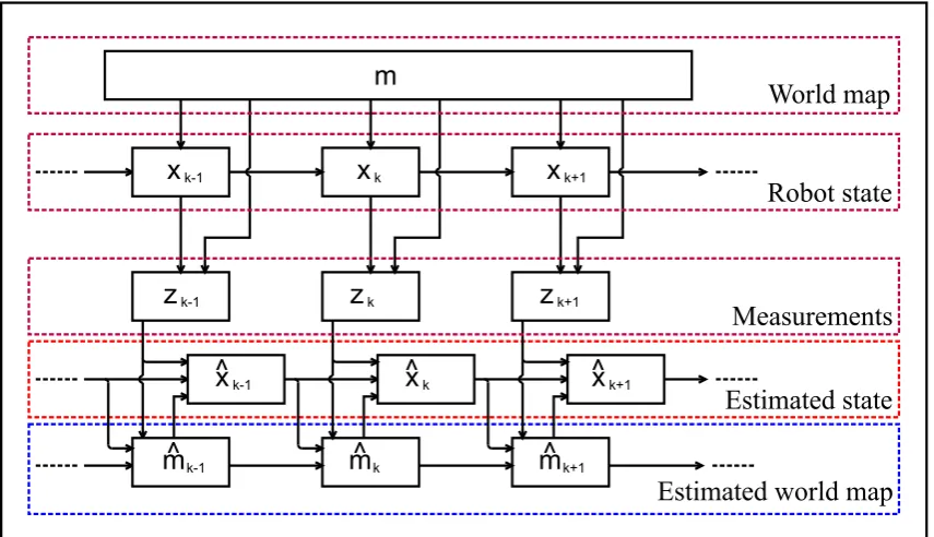
(12) 4. Self Localization of PIRATE Inside a Partially Structured Environment. 2 SLAM: Literature Review and Background Information This chapter introduces the main topic of this research, simultaneous localization and mapping (SLAM). Different SLAM approaches in literature are reviewed and the problem is explained.. 2.1 Basic SLAM problem The aim of SLAM is to detect the state of a robot inside its environment, and to simultaneously make a suitable map of this environment. This in principle is a difficult problem, because to make a good estimate of a robot state, the environment needs to be known, but to make a good estimate of the environment, the robot state needs to be known. Somehow, this must be translated into an iterative process in which a better estimate of the environment leads to a better estimate of the state and vice versa. Figure 2.1 shows a schematic representation of such a process. In this schematic, the robot state (x k ) interacts with the environment (world map m), and the measurements (z k ) are produced as a result of this particular state and environment. Now after each measurement, the estimated map/model of the world is updated from the measurement data and the previous world and state estimates. After that, the state estimate is updated from the same measurement data and the previous state estimate and world estimate. A stochastic approach to obtain a solution to this problem is called recursive bayesian estimation. It is described in the next subsection.. m. World map. x k-1. xk. x k+1. z k-1. zk. z k+1. ^ k-1 x ^ k-1 m. x^ k ^k m. Robot state. Measurements x^ k+1. Estimated state. ^ k+1 m Estimated world map. Figure 2.1: The iterative process of Simultaneous Localization and Mapping. 2.1.1 Recursive Bayesian Estimation To explain Recursive Bayesian Estimation, first the estimation of the environment m is left out. So the problem is to obtain a estimate for the state x k , given the sequence of all measurements Zk = {z 1 , z 2 , . . . , z k }. The state of this system evolves through time according to equation 2.1,. Twan Mennink. University of Twente.

(13) CHAPTER 2. SLAM: LITERATURE REVIEW AND BACKGROUND INFORMATION. 5. in which f k could be a nonlinear function and v k is the process noise. it is assumed that f k is known. x k = f k−1 (x k−1 , v k−1 ). (2.1). Also measurements z k are taken at each sampling interval according to Equation 2.2, in which h k is a known possibly nonlinear function. z k = h k−1 (x k−1 , v k−1 ). (2.2). To obtain an estimate of x k , the posterior p(x k |Zk ), is required, so that for instance the minimum mean-square error (MMSE) estimate of x k can be calculated as in Equation 2.3. Z. E [x k |Zk ] =. x k · p(x k |Zk )d x k. (2.3). The recursive bayesian estimation algorithm consists of a “prediction” step and an “update” step. 2.1.1.1 Prediction Step First the prediction step will be explained. Suppose the pdf p(x k−1 |Zk−1 ) is available. Then the prediction stage involves calculation of p(x k |Zk−1 ), which is done via the Chapman Kolmogorov equation as in Equation 2.4. p(x k |x k−1 , Zk−1 ) reduces to p(x k |x k−1 ), because according to Equation 2.1 the current state x k only depends on the previous state x k−1 and the statistics of v k−1 and not on measurements Zk−1 .. Z. p(x k |Zk−1 ) =. p(x k |x k−1 , Zk−1 )p(x k−1 |Zk−1 )d x k−1 Z. ⇒ p(x k |Zk−1 ) =. p(x k |x k−1 )p(x k−1 |Zk−1 )d x k−1. (2.4). 2.1.1.2 Update Step The update step is now defined by Equation 2.5. The probability density function p(z k |x k ) is derived from the measurement equation 2.2. p(x k |Zk ) =. p(z k |x k )p(x k |Zk−1 ) p(z k |Zk−1 ). (2.5). So by this, the pdf p(x k−1 |Zk−1 ) is evolved to p(x k |Zk ). This provides an analytical method to recursively estimate the state x k of a dynamic system with noise. 2.1.1.3 Analytic Solution In many cases, an analytic solution cannot be found to to the recursive bayesian estimation problem. In case the system dynamics are linear, and both process and measurement noise are additive gaussian, the problem is solved analytically with the Kalman filter. In the nonlinear case, various approximations exist, such as extended Kalman filters, which linearize the system, and particle filters, which use monte carlo integration methods. For further reading on these subjects, Ristic et al. (2004) is an excellent source of information.. Control Engineering. Twan Mennink.

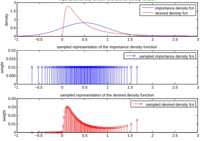
(14) 6. Self Localization of PIRATE Inside a Partially Structured Environment. 2.1.2 Particle Filter A particle filter, (Also called Sampling Importance Resampling filter), is often used in literature to solve a SLAM problem. The operation of such a filter is now explained. First the concept of importance sampling is introduced. 2.1.2.1 Importance Sampling Monte Carlo Sampling is a technique used to approximate a density function f (x) by a finite set of N samples X = {x 1 , x 2 , . . . , x N } with associated weights W = {w 1 , w 2 , . . . , w N }. Given these samples and weights, the function f (x) is approximated by equation 2.6.. f (x) ≈. N X. w i δ(x − x i ). (2.6). i =1. Suppose one wants to evaluate an integral of the form: Z F = g (x) f (x)d x. (2.7). By substituting the sampling approximation for f (x) in Equation 2.7, then an approximation of Equation 2.7 can be found by: " # Z N N X X g (x i )w i (2.8) F ≈ g (x) w i δ(x − x i ) d x = i =1. i =1. Now Suppose a sampled representation of a pdf p(x k |Zk ) is needed. Often one cannot sample directly from that pdf. In case p(x k |Zk ) cannot be sampled directly from, but p(x k |Zk ) can be © ª evaluated for a given x ki , then it is still possible to generate a set of support points x ki , i = 1 . . . N © i ª with associated weights w k , i = 1 . . . N representing p(x k |Zk ). This is done by taking a different © ª pdf q(x k |Zk ) from which samples x ki , i = 1 . . . N are drawn. The weights are now proportional to: p(x ki |Zki ) w ki ∝ (2.9) q(x ki |Zk ) The only prerequisite on q is that it has the same support as p. (p > 0 : q > 0). This method is called importance sampling and q(x k |Zk ) is called the importance density, or in particle filtering, is also often called proposal density. Figure 2.2 shows how the importance sampling works. Samples are drawn from the importance density and all have equal weight. (sum of all weights is one). Now the weights are updated according to Equation 2.9 and are normalized. (total sum is 1). 2.1.2.2 Sequential Importance Sampling Sequential importance sampling makes use of importance sampling to solve the recursive bayesian estimation problem. Let’s say one wants to have a sampled representation of p(X k |Zk ). This can be done by importance sampling, using a proposal density q(X k |Zk ) which factors as: q(X k |Zk ) = q(x k |X k−1 , Zk )q(X k−1 |Zk−1 ) (2.10) Suppose a set of samples drawn from q(X k−1 |Zk−1 ) is already available, and a set of weights i i w k−1 , i = 1, 2, . . . N is also available. The set of weights with the samples X k−1 , i = 1, 2, . . . N is a sampled representation of P (X k−1 |Zk−1 ). The probability density function of the trajectory of x up to time k − 1, given all measurements z up to time k − 1. Ristic et al. (2004) shows that if one now draws samples: X ki ∼ q(x k |X k−1 , Zk ) (2.11) Twan Mennink. University of Twente.

(15) CHAPTER 2. SLAM: LITERATURE REVIEW AND BACKGROUND INFORMATION. Importance density function and desired density function. 2. importance density fcn desired density fcn. 1.5 density. 7. 1 0.5 0 −1. −0.5. 0. 0.5. 1. 1.5. 2.5. 3. sampled representation of the importance density function. 0.02. sampled importance density fcn. 0.015 weight. 2. 0.01 0.005 0 −1. −0.5. 0. 0.5. 1. 1.5. 2.5. 3. sampled representation of the desired density function. 0.04. sampled desired density fcn. 0.03 weight. 2. 0.02 0.01 0 −1. −0.5. 0. 0.5. 1. 1.5. 2. 2.5. 3. Figure 2.2: Example of importance sampling. The desired density is lognormal distributed, the importance density is normal distributed.. and the markov chain order 1 assumption is made, meaning: q(x k |X k−1 , Zk ) = q(x k |x k−1 , z k ). (2.12). Then the new weights w ki , i = 1, 2, . . . N can be calculated: w ki ∝. i p(z k |x ki )p(x ki |x k−1 ). q(x k |x k−1 , z k ). (2.13). This gives a method of taking a previous set of samples and weights, and updating them with new measurement information to a new state. The importance density q(x k |x k−1 , z k ) must be well chosen, because if the density function is too wide for instance, then many samples will get low weights assigned, which makes a poor approximation. Also, one must be able to draw samples from the importance density, as well as evaluate the pdf for that particular sample. So sequential importance sampling gives us a method to get a estimate of the state given all measurements, a problem with this method exists however. It is observed in literature that after only a few time steps, the weights of all particles (or samples) but one will converge to zero. This means that after a few time steps only one particle will be effective. 2.1.2.3 Sequential Importance Resampling The Sequential Importance Resampling (SIR) filter uses sequential importance sampling to solve the recursive bayesian estimation problem. The SIR filter solves the problem of particle degeneracy by resampling after each time step. Resampling is a technique to redistribute all particles according to the existing sampled pdf where more particles are assigned to high probability areas. A high variety of resampling schemes exists in literature, for a variety of situation. A few strategies are: Residual resampling, Stratified resampling and Multinomial resampling. The paper Douc (2005) compares a number of these resampling schemes.. Control Engineering. Twan Mennink.

(16) 8. Self Localization of PIRATE Inside a Partially Structured Environment. 2.2 SLAM state of the art The SLAM problem is a wide topic of ongoing research. The most research done on this subject concerns the 2D SLAM problem, in which a robot moves through a flat 2D environment, for example Grisetti et al. (2007a) and Schroeter and Gross (2008) work on such SLAM type problem. In this 2D world, the robot state is represented by three parameters, namely the coordinates x, y and ϕ. x and y represent the position on the map of the robot, and ϕ represents the orientation of the robot. To represent a map of the environment, an occupancy grid map is often used (Grisetti et al. (2007a), Lu and Milios (1997), Pandey et al. (2007)). This is a grid with cells, and each cell’s value indicates if the cell is occupied or not. Laser range finders are particularly well suited to generate such an occupancy grid. 2.2.1 Sensors Often used for SLAM On most 2D SLAM problems, two types of sensors are used. First, some form of odometry is present, that measures for instance wheel rotations. Secondly, a range finder in some form is often present. Holz et al. (2008) uses a IAIS 3DLS Laser range finder, which is based on the SICK 2D laser range finder. This range finder uses a straight laser line ans scans up and down. Elinas et al. (2006) use a pair of stereo cameras for mapping indoor environments. Fairfield et al. (2006) use a sonar range finder as their main sensor. 2.2.2 Filters Used in SLAM Various types of filters are used in SLAM research, the most notable are particle filters and Extended Kalman filters. If extended Kalman filters are used, a landmark based approach is often used. Landmarks are modeled as coordinates on the map, and their position is then estimated with a certain variance, for instance Newman (1999) uses landmark based maps. Particle filters are more often used in combination with an occupancy grid map. 2.2.3 Map Consistency A SLAM algorithm will have to construct a map consistently. Data from for instance a laser range scanner is combined with odometry data. A problem which is often encountered if all measurements are integrated in a global map, is that this will result in errors accumulating. A straight corridor can become curved, for instance. To overcome this, a map can be restored when a loop in the map is encountered. The algorithm can then correct the map to make sure both measurements of the same locations actually overlap.Lu and Milios (1997) uses such techniques. For these techniques, it is required to keep a trajectory of the robot, and the map as a function of that trajectory. If the trajectory estimate changes, then the map, which is a combination of local maps will also be updated. Another approach is to use some constraints on the map. For instance one could pose the constraint that only 90-degree angles in walls are permitted. This would not require keeping all local maps and trajectories. Rodriguez-Losada et al. (2006) uses geometric constraints to keep the map consistent. 2.2.4 Problem of High Dimensionality In SLAM, the state of the system is the combined state of the robot and the state of the map. Either a grid map or a landmark based map results in a state vector of very high dimensionality. A map can often contain thousands or millions of landmarks, or grid cells. This results in joint probability density functions of very high dimension. In case a particle filter is to be used, it would need a unpractical amount of particles/samples to approximate this high-dimensional joint probability function. One way to overcome this, is to use Rao-Blackwellization. Elinas et al. (2006) uses this, as well as Grisetti et al. (2007b). The objective of SLAM is to estimate the robot trajectory x 1:k and map m, given the sequence all odometry measurements u 1:k and. Twan Mennink. University of Twente.

(17) CHAPTER 2. SLAM: LITERATURE REVIEW AND BACKGROUND INFORMATION. 9. range finder observations r 1:k . This is: p(x 1:k , m|u 1:k , r 1:k ). (2.14). The key aspect of Rao-Blackwellization is to factorize this into: p(x 1:k , m|u 1:k , r 1:k ) = p(x 1:k |r 1:k , u 1:k )p(m|x 1:k , r 1:k ). (2.15). p(x 1:k |r 1:k , u 1:k ) is a localization problem, which is solved by a particle filter, and p(m|x 1:k , r 1:k ) takes the particles of the state trajectories as inputs. The Rao Blackwellized particle filter for SLAM does need to keep a map with every particle though, but this then also has the advantage that multiple hypothesis are kept, so a loop-closing is automatically performed. Only particles which close a loop correctly “survive”, and during a resampling step they will be copied.. 2.3 Conclusions on SLAM in Literature It has been found that many examples exist in literature that solve the 2D, 3DOF SLAM problem satisfactory. Two filtering techniques are most used, Particle filters and Extended Kalman filters. Also, two map representation techniques are most used, occupancy grid mapping and landmark based maps. The main differences between Extende Kalman Filters (EKF) and Particle Filters (PF) are displayed in Table 2.1. In Table 2.2 the differences between Occupancy Grids and Landmark based maps are displayed. To use a landmark based map, often a camera or a camera stereo pair is used to detect SIFT keypoints which are translated into landmarks. The method is less suited if sparse sensor data, from for instance a sonar, or very noisy data is available. PF. EKF. handles complex systems good noise immunity handles non-linear systems Keeps multiple hypothesis High computational costs. Low computational load high demand on noise parameters linearizes system Can lose “track” linear & gaussian: KF=optimal. Table 2.1: Properties of Particle Filters versus Extended Kalman Filters. Occupancy Grid. Landmarks. Fixed spatial resolution Memory fixed no feature recognition required difficult to match subsets. landmarks can be anywhere Memory depends on number of landmarks Must recognize landmark features Easy to match subsets. Table 2.2: Properties of Occupancy grids versus Landmark based maps. Control Engineering. Twan Mennink.

(18) 10. Self Localization of PIRATE Inside a Partially Structured Environment. 3 Design of the Sensor Vessel To perform SLAM inside a small pipe network, a sensor vessel had to be designed and built. This chapter describes the selection of the sensors used on the vessel, and the design of the vessel itself.. 3.1 System description The task of the sensor vessel is to move through a straight section of pipe, and to map the location of features like bends and T-junctions. This is the first step towards a fully autonomous PIRATE pipe inspection robot. It is likely that in the future a new version of the PIRATE prototype will be built. It has to be taken into account that the sensors, hardware and software used are suitable for implementation on a stand-alone low-power platform. The focus of this research is to develop algorithms for performing SLAM in a pipe network, therefore it is not required that the processing is done embedded. It is chosen to divide the entire sensing system to perform SLAM into three parts. Hardware, Data-acquisition and SLAM algorithm. Figure 3.1 shows the overview of this system. The function of each part is described in Table 3.1. In the next sections, the design of these three parts is described.. Hardware. Data acquisition. SLAM Algorithms. Figure 3.1: Overview of the system design. Component:. Function. Hardware Data-acquisition SLAM Algorithms. To move through a straight section of pipe, and generate sensor data. To read the sensor data, to present the data to the SLAM Algorithms To localize the vessel inside the pipe, to map the pipe features.. Table 3.1: Function of the different components of the sensing system. 3.2 Hardware Design The hardware of the sensing system consists of a mechanical setup which holds all sensors used, and is able to move through the pipe, and the sensors itself with interfacing electronics. First the selection of the different sensors used is described. 3.2.1 Sensor Selection As pointed out in Subsection 2.2.1, sensors used for SLAM are often a combination of a visual type sensor such as a laser range finder and odometry such as wheel encoders. For this project, it is chosen to use three types of sensors. A Laser range finder, a rotary wheel encoder and a Inertial Measurement Unit. When moving inside a straight pipe, these three sensors combined can be used to obtain a state estimate. 3.2.1.1 Laser Range Finder A laser range finder is a sensor which emits a laser pattern, and using a optical sensor such as a camera, detects the location of this pattern in 3D. In most 2D SLAM applications, the laser range finder is pointed at the floor ahead of the robot, to detect obstacles which are placed on that floor. Inside a pipe, however, there is no floor. The system needs to scan the entire pipewall for obstacles or features. Drost (2009) has built such a system at our laboratory. It is a laser range scanner which projects a circle on the pipe wall. This system still has some drawbacks, Twan Mennink. University of Twente.

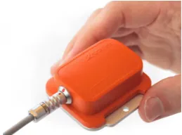
(19) CHAPTER 3. DESIGN OF THE SENSOR VESSEL. 11. most notably are its physical size and the speed of the data processing. Therefore, this sensor is redesigned. A detailed description of the redesign can be found in Chapter 4. If the sensor is placed inside a perfectly round, straight section of pipe, then the sensor provides enough information to detect the pose of the sensor with respect to the pipe axis. However, it cannot detect rotations around the pipe axis, and also cannot detect translational motion along the pipe axis. 3.2.1.2 Inertial Measurement Unit To overcome the problem of not being able to detect rotations around the pipe center axis, a inertial measurement unit is added to the sensor array. The sensor used is a Xsens MTi. (www.xsens.nl). This sensor has the capability estimating its entire orientation, but this relies on the earth-magnetic field. Inside the gas network, which may be metal pipes, this will not work properly. Also, the PIRATE Mainboard contains acceleration sensors. It is therefore chosen to only use the acceleration data of the Xsens unit. This makes the sensing system more compatible with future PIRATE designs. Using the acceleration data, now a distinction can be made between two orientations which are rotated around the pipe axis. Figure 3.2 shows a photo of this sensor.. Figure 3.2: Xsens MTi Inertial Measurement Unit (IMU). 3.2.1.3 Rotary Wheel Encoder To be able to also measure translational motion along the pipe axis, a optical encoder is fitted to one of the wheels of the sensor vessel. Now three sensors are available which make it possible to sense all vessel states inside a straight pipe. Figure 3.3 shows the location of the wheel encoder.. 1. 2 3. Figure 3.3: Sensor vessel outside pipe with 1: Wheel encoder, 2: IMU, 3: Laser range finder. Control Engineering. Twan Mennink.

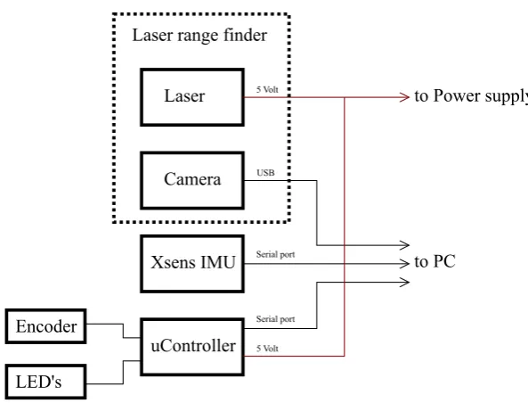
(20) 12. Self Localization of PIRATE Inside a Partially Structured Environment. 3.2.2 Mechanical Design of the Sensor Vessel A prototype style sensor vessel has been built for this project. As said, the sensor vessel contains a Inertial Measurement Unit (IMU), one wheel is equipped with an optical encoder and a custom built laser range finder built upon the work of Drost (2009). A few pictures of the built vessel can be seen in Figure 3.3 and Figure 3.4. The chassis of the sensor vessel of made to hold all the sensors. A very basic design is chosen, the chassis just consists of a piece of PVC pipe. The suspension has been made such, that the vessel approximately centers itself inside a pipe. The minimum diameter of pipe in which this vessel fits is 120[mm].. Figure 3.4: Photographs of the sensor vessel inside the pipe,where the suspension is fully impressed.. 3.2.3 Interface electronics The interfaces of the sensor vessel to the outside world are shown schematically in Figure 3.5. A personal computer connects with two serial ports and one USB port to the vessel. The custom made serial communication protocol with the microcontroller is described in Appendix B.1.. Interfaces of the Sensor Vessel. Laser range finder Laser. 5 Volt. Camera. USB. Xsens IMU Encoder. Serial port. to Power supply. to PC. Serial port. uController. 5 Volt. LED's Figure 3.5: The interfacing between the sensor vessel and PC. Twan Mennink. University of Twente.

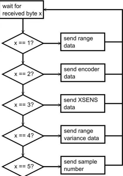
(21) CHAPTER 3. DESIGN OF THE SENSOR VESSEL. 13. 3.3 Data Acquisition Software The data acquisition software is the piece of software which reads out all sensors on the sensor vessel, and presents this data in a structured manner to the SLAM algorithm. It is chosen the divide the data acquisition software into a server and client which communicate via a TCP/IP network connection. The function of the server is to communicate with the various sensors, and to give this data in a simple manner to the client. The function of the client is to receive the data from the server and to present it to the SLAM algorithm in a struct. Figure 3.6 shows the connection in this data acquisition software. Sensor 1. protocol 1. Data acquisition server -communicate with sensors -gather data -transmit data. Sensor n. Data acquisition client -receive data -order data in struct. protocol n. tcp/ip comm to SLAM algorithm data 1 struct data 2 ...... data n Figure 3.6: Schematic representation of the function of the data acquisition software. 3.3.1 Basic Operation of the Data Acquisition Server The data acquisition server makes use of different threads to do its tasks. A total of four processes run simultaneous. The function of the threads are: • Image processing: Read frames from camera and extract the laser curve in polar coordinates. • Xsens: Continuously receive the Xsens data and place in a fifo buffer. Analyse buffer content for valid data frames. • Microcontroller: Wait for data from encoder readout. • UDP Server: The network thread, which waits for messages from the client. So the threads continuously gather data from the sensors, and when a client asks for data, the server gives the most up-to-date sensor values. A detailed description of the threads used and the different classes can be found in Appendix B.2. Figure 3.7 shows the basic communication between the server and the client. 3.3.2 Data Acquisition Client The client which calls the server periodically for sensor data is implemented in Matlab. Matlab has some built in functions to handle network UDP traffic, so these functions are used. The communication protocol between the client and the server is very basic. The client sends a one-byte value, ranging from 1 to 5, which indicates the type of data requested. The server then responds with a message with the raw data. No frame headers or such are used. The data-acquisition client also uses calibration data to calculate 3D information from the polar coordinate laser range finder data. This is done by a mapping table and details about this can be found in Chapter 4. The source code of the data acquisition client can be found in the files listed in Table G.2. The program is started by running getNetwork.m, listed in Table G.2. The program will store all measured data in a struct array “Sample”, containing the entries shown in Table 3.2:. Control Engineering. Twan Mennink.

(22) 14. Self Localization of PIRATE Inside a Partially Structured Environment. wait for received byte x. x == 1?. send range data. x == 2?. send encoder data. x == 3?. send XSENS data. x == 4?. send range variance data. x == 5?. send sample number. Figure 3.7: Basic mode of operation of the UDP server. A thread from the main program continuously listens for data and replies.. struct entry:. description:. x y z R std s. calculated world x-coordinates, laser range finder [mm] calculated world y-coordinates, laser range finder [mm] calculated world z-coordinates, laser range finder [mm] vector with the acceleration data from Xsens [m/s 2 ] standard deviation of laser range finder datapoints [pi xel s] encoder counter value, calculated in mm of travel [mm]. Table 3.2: Description of the struct array Sample, containing pre-processed measurement data. 3.4 SLAM Algorithm The slam algorithms used in the sensing system is a combination of vessel state estimation using a particle filter, and a pipe map algorithm using a variation to the occupancy grid. The design and implementation of these algorithms are described in Chapter 5. 3.5 Conclusions In this chapter, the overall design of the sensor vessel with the used software is described. Now a sensor vessel is available with data acquisition software which presents data for the SLAM algorithms in a structured manner. In Chapter 4 the details of the redesign of the Laser range finder is described, and in Chapter 5 the design of the actual SLAM algorithm is described.. Twan Mennink. University of Twente.

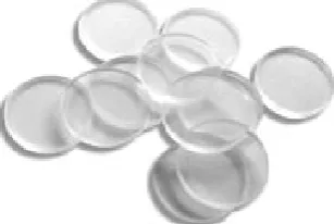
(23) 15. 4 Redesign of the Laser Range Finder This chapter describes the redesign and implementation of the hardware and software of the laser range finder. First the upgrade of the hardware is described. After that an analysis is made of the optimal setup for the sensor. The sensing system also consists of a software processing part. These parts are described in Section 4.3 Furthermore the Calibration of the sensor is described in Section 4.4. Finally the correct working of the sensor is verified in Section 4.5.. 4.1 Hardware Optimization of the Optical Sensor The optical system to measure pipe profiles Drost (2009), is chosen as a basis for this project’s laser range finder. This system however, has to be redesigned somewhat to become suitable for the new sensor platform. The existing system by Drost (2009) is shown in Figure fig:opticalsetup. The size of the sensor system needs to be made smaller, and it is preferred to eliminate the moving parts of the system. Also, the processing algorithms need to be less time consuming.. Rotating mirror. Laser. Laserbeam. 100. Motor. Camera. Figure 4.1: The optical setup as designed by Drost (2009). 4.1.1 Elimination of Sensor Moving Parts The moving parts of the optical sensor system consist of the fast rotating, titled, mirror which forms the basis of the cone projection. Fortunately this part can be replaced by a passive element, called a Diffractive Optical Element (DOE). Such an element is based on diffraction of the laser beam to create a circle shaped diffraction pattern. The setup built in this project is using a standard Diffractive Optical Element manufactured by Holo-eye (http://www.holoeye.com). This element projects a circle on a flat surface, with a radius that linearly depends on the distance to the surface. Figure 4.2 shows what these Diffractive Optical Elements look like.. Figure 4.2: Sample photograph of Diffractive Optical Elements. Control Engineering. Twan Mennink.

(24) 16. Self Localization of PIRATE Inside a Partially Structured Environment. 4.1.2 Replacing Camera and Alterations to the Lens For the Sensor Vessel, the old camera was not suitable because its size is not suitable for placement inside the vessel chassis. A camera with a different physical geometry is chosen to overcome these problems. In Figure 4.3, the new camera is shown which has a cylindrical shape, and the old camera has a more flat shape. The cylindrical shape is better suited for this application because now the laser beam which is coming from behind the camera is not blocked by the camera body. After the new camera was tested, it was concluded that the angle of view was not large enough. This was solved by adding a fish-eye lens to the camera.. (a) Old camera. (b) New cylindrical shaped camera. Figure 4.3: Picture of the old and the new camera. 4.2 Optical Sensor Configuration Analysis The optical pipe profiling system uses triangulation methods with structured light to obtains 3D information about the environment. Figure 4.4 shows a possible configuration of this system. In this section it is analyzed how different parameters of the setup influence overall performance of the system. This is done by taking a finite number of coordinate points which lie on the laser cone surface, and calculating what the camera pixel coordinates for these coordinate points will be. From this data, it can be assesed what the theoretical resolution and range of the system will be. A number of configurations will be simulated this way, to find the most feasible configuration.. Laserbeam. camera projector. Figure 4.4: A simple representation of a possible configuration of the pipe profiling system. 4.2.1 Mathematical framework This subsection describes the mathematical framework used for the analysis. First the camera is described and after that, the Projected laser cone is described.. Twan Mennink. University of Twente.

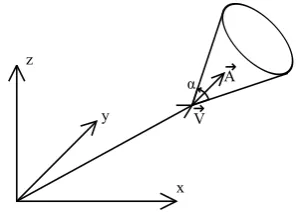
(25) CHAPTER 4. REDESIGN OF THE LASER RANGE FINDER. 17. 4.2.1.1 Camera Model For this analysis, the camera is modelled as an ideal pinhole camera. Such a camera can be ~ . R and fully described by a calibration matrix K , a rotation matrix R and a translation vector T ~ T describe the orientation and position of the camera with respect to the fixed world coordinate system. The calibration matrix K describes the conversion between 3D points in camera ~w in world coordinates to 2D points on the camera projection plane. So if we now have a point P ~c is, coordinates, and we want to know where the corresponding point in camera coordinates, P we get: ¡ ¢ ~c = R P ~w − T ~ P (4.1) If it is assumed that the pixel size of the camera is exactly square everywhere, and that the image plane is exactly centered around the pinhole of the camera, then the calibration matrix K becomes:   f ·s 0 0 f · s 0 K = 0 (4.2) 0 0 1 In which f is the focal distance, or the perpendicular distance between the image plane and the pinhole, and s is a scaling factor which represents the number of pixels per metre on the image plane. From this it is easy to see that the horizontal (u) and vertical (v) pixel coordinates of the image will become: xc · f ·s zc yc · f ·s v= zc. u=. (4.3) (4.4). This concludes the mathematical camera model. 4.2.1.2 Laser Cone model A cone which is centered around a coordinate axis can easily be described by using cylindrical coordinates. If the cone for instance is aligned with the z axis, then using cylindrical coordinates (r ,θ,z) this becomes: r =k ·z (4.5) In order to calculate a finite number of points along the cone’s surface, a parametric equation is made which describes a spiral along the cone’s surface. α is defined as the opening angle of the cone. α ·z 2 θ =K ·z r = tan. (4.6) (4.7). This can be converted into carthesian coordinates to get: α · z · cos(K · z) 2 α y(z) = tan · z · sin(K · z) 2. x(z) = tan. (4.8) (4.9). The parametric cone equation can be translated and rotated to get any desired cone in 3D ~ describes the origin of the cone space. Figure 4.5 shows this representation, in which vector V ~ and vector A describes the direction of cone. The original cone equation points towards the z axis, so to transform this by means of a rotation matrix R c to a cone pointing in the direction of A A, at least the third column of this matrix should be the unit vector |A| . The cone is invariant to rotations around the axis A, so the only restriction on the first and second columns of R c are Control Engineering. Twan Mennink.

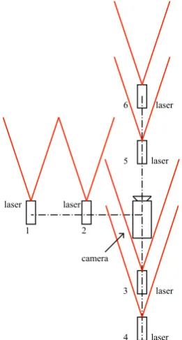
(26) 18. Self Localization of PIRATE Inside a Partially Structured Environment. z. A. α y. V. x. Figure 4.5: Cone description in 3D space.. ~ , this can be that they are perpendicular to both themselves and A. If we take a random vector B achieved as follows: ~ r3 = ~ Aˆ. (4.10). ~ ×~ B r3 ~ r2 = ¯ ¯ ¯B ~ ×~ r3¯. (4.11). ~ r 1 =~ r 2 ×~ r3 £ ¤ r1 ~ r2 ~ r3 Rc = ~. (4.12) (4.13). ~ , the coordinates of a point p cone ~ on the cone surface can be Using this matrix and the vector V transformed into world coordinates by: ~wor l d = R c · p ~cone + ~ p v. (4.14). In Appendix A.1, a Matlab script is given which calculates points along a desired cone surface, at a certain interval (distance between points). The output result of this script is shown in Figure 4.6.. 0.35 z axis. 0.3 0.25 0.2 0. 0.15 −1.7. 0.1 −1.8 −1.9 y axis. 0.2 −2. x axis. Figure 4.6: Cone output of matlab script. 4.2.2 Numerical Simulation of Camera Images In this subsection, a numerical simulation of the camera images produces by different configuration is described. This simulation is made by first calculating a large amount of points on Twan Mennink. University of Twente.

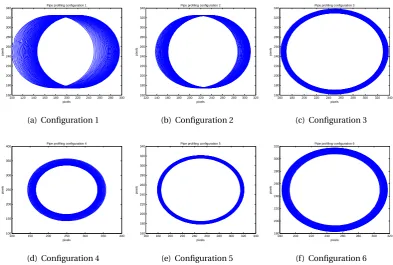
(27) CHAPTER 4. REDESIGN OF THE LASER RANGE FINDER. 19. the surface of the laser cone (Appendix A.1), and then the ideal pinhole camera image of these points is calculated. A total of six configurations will be simulated here. Figure 4.7 shows the different configurations which are simulated here.. 6. 5. laser. laser. laser. laser 1. 2 camera 3. 4. laser. laser. Figure 4.7: Different simulated configurations of the optical sensor. The opening angle of the cone is set such that a circle with diameter of 60mm will be projected at 100mm distance. (this specific opening angle is taken from the Diffractive optical element specifications). The positions of the projector with respect to the camera pinhole are as in Table 4.1. Config nr:. x pos. z pos. 1 2 3 4 5 6. -5 [cm] -2.5 [cm] 0 [cm] 0 [cm] 0 [cm] 0 [cm]. 0 [cm] 0 [cm] -2.5 [cm] -5 [cm] 2.5 [cm] 5 [cm]. Table 4.1: Position of projector with respect to camera pinhole. 4.2.2.1 Results of the Numerical Simulation The results of the numerical simulations are shown in figure 4.8. As can be seen, in case the cone projector is not on the optical axis, as in configurations 1 and 2, the mapping from points on the cone to camera coordinates is not one-to-one. This means that for some camera coordinates, there are multiple world coordinates associated with that point. It can easily be shown that this only happens when the camera pinhole is located outside the cone. If the camera pinhole is behind the cone, then a one-to one mapping is also possible, but only if the camera is inside the virtual ’mirror’ cone. (The invisible section of cone behind the origin of the projected cone). The simulations show that there is a bigger difference between largest and smallest diameter if the projector is at a distance away from the camera pinhole. Configurations 4 and 6 are better in this property than configurations 3 and 5. Of course if the projector would be located at the camera pinhole, then there would be no difference at all between small and large Control Engineering. Twan Mennink.

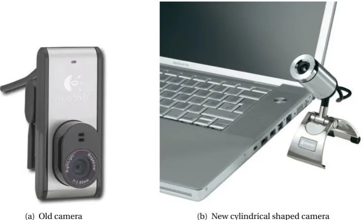
(28) 20. Self Localization of PIRATE Inside a Partially Structured Environment. Pipe profiling configuration 1. Pipe profiling configuration 2. 340. 320. 300. 300. 300. 280. 280. 280. 260. 260. 260. pixels. 320. 240. 240. 240. 220. 220. 220. 200. 200. 200. 180. 180. 160 100. 120. 140. 160. 180. 200 pixels. 220. 240. 260. 280. 160 120. 300. 180. 140. (a) Configuration 1. 160. 180. 200. 220 pixels. 240. 260. 280. 300. 160 160. 320. (b) Configuration 2. Pipe profiling configuration 4. 400. Pipe profiling configuration 3. 340. 320. pixels. pixels. 340. 200. 220. 240 260 pixels. 280. 300. 320. 340. (c) Configuration 3. Pipe profiling configuration 5. 340. 180. Pipe profiling configuration 6. 320. 320. 300. 350 300. 280 280. 250. 200. 260. 260. pixels. pixels. pixels. 300. 240. 240. 220 220 200. 150. 200. 180 100 100. 150. 200. 250 pixels. 300. 350. 400. (d) Configuration 4. 160 160. 180. 200. 220. 240 260 pixels. 280. 300. 320. 340. 180 180. 200. 220. 240. 260. 280. 300. 320. pixels. (e) Configuration 5. (f) Configuration 6. Figure 4.8: Numerical simulation output of configurations 1,2,3,4,5 and 6.. diameters. If the projector is placed too far in front of the camera, almost difference will be present. If the projector is placed too far back of the camera, then the desired diameters to measure will be out of the field of view of the camera. The influence of varying this parameter is shown in Figure 4.9. Diameter measurement range versus position of projector. range [pixels]. 150. 100. 50. 0 −0.15. −0.1. −0.05. 0 0.05 Position of projector [m]. 0.1. 0.15. 0.2. Figure 4.9: Influence of varying the projector position along the optical axis of the pinhole camera. If projector origin is at the pinhole, no triangulation is possible.. 4.2.3 Conclusions of the Laser Range Finder Analysis In this subsection a quantitative analysis has been done of the pipe profiling measurement system. It is argued that for a one-to-one mapping of world coordinates lying on the cone, to camera pixel coordinates, the camera pinhole should be inside the cone, or inside the virtual mirror opposite of the cone (negative z-coordinates in equation 4.9). For equal dynamic range in all directions, it is desirable to place the projector onto the optical axis of the camera, and also have the projector point into the same direction as the camera. The best position for optimal dynamic range would be to place the projector behind the camera. This concludes the analysis of the optical measurement system.. Twan Mennink. University of Twente.

(29) CHAPTER 4. REDESIGN OF THE LASER RANGE FINDER. 21. 4.3 Processing of the Image Data This section will discuss the procedure to obtain the desired 3D information from the structured light optical sensor system. The processing method used by the system built by Drost (2009) is looked at, and also alternative methods are compared. 4.3.1 Common Procedure for 3D Information Retrieval In common, the retrieval of 3D information from structured light projection images taken by a camera, is involving some sort of laser curve extraction algorithm, a formula for calculation of 3D coordinates from image coordinates and some form of calibration data. These procedures will now be discussed. 4.3.1.1 Laser Curve Extraction Methods The first step in measuring, is to extract the pixels from the camera image that belong to the laser curve. The method used by Drost (2009) consist of five steps, which are shown briefly in Figure 4.10(a). Furthermore, Duran et al. (2003) use a approach which is a bit different, by first fitting an ellipse to the data. Their method is shown in Figure 4.10(b). This is because Duran wants to find defects on the pipe wall, and Drost needs to map the entire pipe wall. Drost’s method would be suitable for this project, only the speed of the algorithm is not fast enough. Therefore it was chosen to try a different approach. The next subsection will describe this new approach. Start. Start. Start. Median Filter. Median Filter and Intensity norm.. Polar Mapping. Image Segmentation. Ellipse Curve Fitting 1D Column Fitering. Image Segmentation Along ﬁtted curve Object Selection. Object Selection. Subpixel curve detection. (a) Drost’s method to extract the laser curve.. Feature Extraction. (b) Duran’s method to extract the laser curve.. Subpixel curve detection. (c) New approach to extract the laser curve.. Figure 4.10: Different image processing approaches for extracting laser curves.. 4.3.1.2 New Approach to Laser Curve Extraction This subsection describes the new approach of laser curve extraction, which makes use of the fact that all image data is radially oriented around some center point which is the camera image of the center axis of the cone. The assumption is made here that the camera image of center of the cone does not move much as a function of distance. (This is true only if the projector is aligned exactly with the optical axis of the camera). The new approach will make a polar coordinate mapping of the image around the center point. Part of the calibration data will thus be obtaining this center point (x 0 , y 0 ). This mapping is shown in equations 4.16.. Control Engineering. Twan Mennink.

(30) 22. Self Localization of PIRATE Inside a Partially Structured Environment. q (x − x 0 )2 + (y − y 0 )2 y − y0 φ = at an x − x0. r=. (4.15) (4.16). As an example, the resulting transform of the image in Figure 4.11(a) looks like the image in Figure 4.11(b). The advantage of having this representation, is that because of approximately radial orientation of the original image, the laser can be found in the vertical direction on every column. This makes finding the laser curve a one-dimensional search problem on every column. It is assumed that the laser curve will have a Gaussian radial intensity, so the search algorithm will need to find the peak of a Gaussian shape in each column. Finding this Gaussian peak will be done by first smoothing the data with a vertical blur on each column and then apply a 1D Laplacian of Gaussian function to the image. The blur and second-derivative of Gaussian convolution kernels can be combined into one single kernel. The Gaussian blur function is shown in Equation 4.17, the second derivative function is shown in Equation 4.18. The realization of these kernels can be shown in Figure 4.12. When these are applied to the image of Figure 4.11(b), the resulting image is shown in Figure 4.22. The minimum value of each column now represents the location of the laser curve. Using a weighted average around the pixel with minimum intensity will give sub-pixel accuracy to this measurement. 4.3.1.3 Comparison of new Laser Curve Extraction with Existing Algorithm To compare the proposed laser curve extraction algorithm with the existing one by Drost (2009), both are tested on the same computer. Performance is measured by using the Matlab Profiler tool, the time duration of every step is recorded. The most significant steps are listed in Table 4.2. The new approach is faster by almost a factor of 10. After inspection of the segmentation algorithm, it is found that a lot of nested loops are present in this algorithm. These probably cause the long calculation time of this part. A remark must be made however, that the relative accuracy of the algorithms are not easy to obtain because the algorithms are both written to different hardware used with different calibration procedures.. (a) Example image to describe the laser curve extrac- (b) Polar coordinate transform of the example image. tion.. Figure 4.11: Example of transforming image with polar coordinate mapping.. .. (x−µ)2 1 − f (x) = p · e 2·σ2 2πσ2. (4.17). µ ¶ (x−µ)2 1 (x − µ)2 1 − gx = p · e 2·σ2 · + σ4 σ2 2πσ2. (4.18). Twan Mennink. University of Twente.

(31) CHAPTER 4. REDESIGN OF THE LASER RANGE FINDER. 23. gaussian blur convolution kernel, σ = 5, µ = 50.5 0.08. y axis [ ]. 0.06 0.04 0.02 0. 0. 10. 20. 40. 50 60 x axis [pix]. 70. 80. 90. 100. 90. 100. Laplacian of gaussian convolution kernel, σ = 5, µ = 50.5. −3. 2. 30. x 10. y axis [ ]. 1 0 −1 −2 −3 −4 0. 10. 20. 30. 40. 50 60 x axis [pix]. 70. 80. Figure 4.12: Convolution kernels for detection of laser Edge.. (a) Preprocessed and filtered image. (b) Filtered image, with extracted laser curve. Figure 4.13: This Figure shows the image from Figure 4.11(b), but now it is filtered with the kernel from equation (4.17) and then filtered with the kernel from equation (4.18). In (b), the detected laser curve is also added.. (a) Time duration Drost algorithm. (b) Time duration new approach. Program step. Time used. Program step. Time used. Median filter Segment Image Select objects total time. 0.929[s] 6.149[s] 1.16 [s] 8.241 [s]. Polar transform Filter image Select objects total time. 0.460 [s] 0.411 [s] 0.03 [s] 0.874 [s]. Table 4.2: (a):Time duration of the most significant steps in the laser curve extraction algorithm by Drost. (b)Time duration of the most significant steps in the approach used in this research. (Hardware, Pentium 4-2600 Mhz, 1.5 Gb RAM). 4.3.1.4 Retrieval of 3D Information from Extracted Laser Curve This subsection describes the methods used and in particular the method used for this research to retrieve the 3D information from the extracted laser curve. Basically, there are two methods to retrieve 3D information. In literature, the 3D information is often retrieved by using a mathematical model of the camera and the projector, and a list of calibrated model parameters. Zhang (1999), Reilink (2008), Drost (2009) and Duran et al. (2003) all use this method. Perwass and Sommer (2006) use a bit different version of a camera model, but still rely on the use of a model to retrieve 3D information. Another way of retrieving 3D information from camera pixel locations is by making a lookup table between the pixels and the points in 3D space. Interpolation can then be used to obtain 3D information for the entire domain. Such an approach is used. Control Engineering. Twan Mennink.

(32) 24. Self Localization of PIRATE Inside a Partially Structured Environment. by for instance Wu1 and Tsai1 (2009). In their paper, they make a lookup table for world coordinates lying on a plane perpendicular to the camera optical axis at a certain distance. They are using analytical methods to adapt this table for a camera at different orientations and/or distances. This means that the camera orientation needs to be known. 4.3.1.5 Retrieval of 3D data using lookup Table For this research, the lookup table method is chosen, because this method has low complexity, and requires little calculation. This is beneficial if implementation onto an embedded target system is required. For this method to be applied, a number of points on the cone surface are mapped to unique camera pixel coordinates. This mapping is recorded using the calibration procedure described in the next Section. The cone projected by the laser is actually a 2D surface. Therefore, the mapping needed is also from ℜ2 to ℜ2 . How this mapping is made exactly is shown in Subsection 4.4.2.6.. 4.4 Calibration of the Optical Setup This section describes the calibration method of the optical sensor. Conventionally, a camera is calibrated by estimating the intrinsic and extrinsic camera parameters (for instance, Zhang (1999)). On top of this, the nonlinear lens distortions must also be estimated (See Reilink (2008) and also Zhang (1999)). The result of such a calibration will be that captured images captured can be transformed in such a way, that it seems as if the picture was taken by an ideal pinhole camera with known intrinsic and extrinsic parameters. 4.4.1 Disadvantages of Conventional Calibration For the conventional camera calibration method, it is required to have a fairly good model of the camera and lens behaviour. This setup however, contains a large number of components with poor specifications available. It was observed by rotating the camera lens for instance that the fish-eye lens is not exactly located in the center of the camera. Also the alignment between the laser projector and camera are not easily measured. It is estimated that using a conventional calibration method will give poor estimations because a lot of unmodeled behavior. 4.4.2 New Calibration Method For the 3D acquisition procedure used described in section 4.3.1.4, it is not necessary to have estimates of the camera parameters. The only data required is a mapping function which maps camera pixels to points on the surface of the projected cone. This is determined by using known points on the surface of the cone and finding the image location of these known points. Using interpolation, a complete map of the locations inbetween these points can be made. 4.4.2.1 Calibration Points on the Projected Cone For the calibration, first a number of predefined points on the surface of the cone are defined. On the cone surface a number of conic sections are taken, perpendicular to the cone axis. These sections are circles, which have a diameter varying from 70mm until 135 mm with steps of 5mm. On each circle, 18 points are selected, equally spaced every 20 degrees. For example, on 70 the first ring, the first point will be at coordinate x = 70, y=0 z = t an(α) . (alpha is the opening angle of the cone, as in Equation 4.7). In Figure 4.14 the points used for Calibration are displayed in a 3D frame. 4.4.2.2 Referencing the Calibration Points Now a method of recording these points needs to be found. This is done by placing a flat surface exactly perpendicular to the projector axis, at the predefined distances from the cone origin. This will result in a circle of required diameter to be projected onto the flat surface. Now a. Twan Mennink. University of Twente.

(33) CHAPTER 4. REDESIGN OF THE LASER RANGE FINDER. 25. Calibration points on cone surface. y axis [mm]. 100 50 0 −50 −100. −100 −50. 400 0. 300 50. 200. 100 x axis [mm]. 100 z axis [mm]. 0. Figure 4.14: The points on the cone used for calibration. reference point on the circle needs to be defined, for the 18 points onto the circle to have a common starting point. Figure 4.15 shows what the projected circle looks like. Three small sections of the circle are not lit, this is because the construction of the sensor vessel still needs an optimization. These sections can now be exploited, to have a common starting point for the 18 points on each circle. The location of these 18 points are drawn as blue circles in Figure 4.15. The arrow with the word “reference” points towards the end of the laser gap, which is the location of the first point.. reference. Figure 4.15: Laser cone projected on a flat surface perpendicular to cone, with reference marked, and locations of the 18 points along the circle also marked.. 4.4.2.3 Projector Calibration Hardware To record a set of points on the perpendicular plane, first the laser projector axis needs to be aligned exactly perpendicular to the projection plane. This is done by building a piece of calibration hardware which holds the sensor vessel, contains an adjustable projection plane, and the distance between the projector and this plane is variable. Figure 4.16 shows this setup.. Control Engineering. Twan Mennink.

(34) 26. Self Localization of PIRATE Inside a Partially Structured Environment. up. Sensor vessel. down. Laser cone. Adjustable platform. (a) Schematic display of the calibration hard- (b) Photo of the calibration hardware, the senware. sor vessel is held by a clamp.. Figure 4.16: The calibration hardware, the height of the projector is adjustable, the ground plane’s orientation is also adjustable. 4.4.2.4 Aligning the Projector with Projection Plane As told, the projector axis needs to be perpendicular to the projection plane. The hardware is built such, that the plane can be adjusted by adjusting the length of the three bolts supporting the plane. The procedure to make the plane perpendicular to the projector axis is to use a cylindrical piece of alignment tube which has a line printed on the inside. When the laser beam is exactly aligned with the line on the inside wall of the tube, then the plane is perpendicular to the projector axis. The alignment tube is shown in Figure 4.17. The alignment could also be done by printing a circle on a piece of paper, but using this vertical tool makes the sensitivity for misalignment much larger. After the projection plane is properly aligned, the height adjustment knob of the setup can be used to adjust the radius of the projected circle on the plane.. Figure 4.17: Cylinder shape used to assist in aligning the Projection plane with the projector.. Twan Mennink. University of Twente.

No results found