Power output by an asynchronous flight muscle from a beetle

Animals have evolved two rather different solutions to the task of providing muscles that can operate at high contraction

frequencies: a quantitative solution, which is based on the speeding up of time-consuming steps in muscle activation and JEB2869

The basalar muscle of the beetle Cotinus mutabilis is a large, fibrillar flight muscle composed of approximately 90 fibers. The paired basalars together make up approximately one-third of the mass of the power muscles of flight. Changes in twitch force with changing stimulus intensity indicated that a basalar muscle is innervated by at least five excitatory axons and at least one inhibitory axon. The muscle is an asynchronous muscle; during normal oscillatory operation there is not a 1:1 relationship between muscle action potentials and contractions. During tethered flight, the wing-stroke frequency was approximately 80 Hz, and the action potential frequency in individual motor units was approximately 20 Hz. As in other asynchronous muscles that have been examined, the basalar is characterized by high passive tension, low tetanic force and long twitch duration.

Mechanical power output from the basalar muscle during imposed, sinusoidal strain was measured by the work-loop technique. Work output varied with strain amplitude, strain frequency, the muscle length upon which the strain was superimposed, muscle temperature and stimulation frequency. When other variables were at optimal values, the optimal strain for work per cycle was approximately 5 %, the optimal frequency for work per cycle approximately 50 Hz and the optimal frequency for mechanical power output 60–80 Hz. Optimal strain decreased with increasing cycle frequency and increased with muscle temperature. The curve relating work output and strain was narrow. At frequencies approximating those of flight, the width of the work versus strain curve, measured at half-maximal work, was 5 % of the resting muscle length. The optimal muscle length for work output was shorter than that at which twitch and tetanic tension were maximal. Optimal muscle length decreased with increasing strain. The curve relating work output and muscle length, like that for work versus strain, was narrow, with a half-width of approximately 3 % at the normal flight

frequency. Increasing the frequency with which the muscle was stimulated increased power output up to a plateau, reached at approximately 100 Hz stimulation frequency (at 35 °C). The low lift generated by animals during tethered flight is consistent with the low frequency of muscle action potentials in motor units of the wing muscles. The optimal oscillatory frequency for work per cycle increased with muscle temperature over the temperature range tested (25–40 °C). When cycle frequency was held constant, the work per cycle rose to an optimum with increasing temperature and then declined. We propose that there is a temperature optimum for work output because increasing temperature increases the shortening velocity of the muscle, which increases the rate of positive work output during shortening, but also decreases the durations of the stretch activation and shortening deactivation that underlie positive work output, the effect of temperature on shortening velocity being dominant at lower temperatures and the effect of temperature on the time course of activation and deactivation being dominant at higher temperatures.

The average wing-stroke frequency during free flight was 94 Hz, and the thoracic temperature was 35 °C. The mechanical power output at the measured values of wing-stroke frequency and thoracic temperature during flight, and at optimal muscle length and strain, averaged 127 W kg−1muscle, with a maximum value of 200 W kg−1. The power output from this asynchronous flight muscle was approximately twice that measured with similar techniques from synchronous flight muscle of insects, supporting the hypothesis that asynchronous operation has been favored by evolution in flight systems of different insect groups because it allows greater power output at the high contraction frequencies of flight.

Key words: asynchronous muscle, work, power, beetle, Cotinus mutabilis, insect, flight.

Summary

Introduction

POWER OUTPUT BY AN ASYNCHRONOUS FLIGHT MUSCLE FROM A BEETLE

ROBERT K. JOSEPHSON1,*, JEAN G. MALAMUD1 ANDDARRELL R. STOKES2

1_{School of Biological Sciences, University of California, Irvine, CA 92697, USA and} 2_{Department of Biology,}

Emory University, Atlanta, GA 30322, USA

*e-mail: [email protected]

relaxation, and a qualitative solution in which some of the time-consuming steps are totally bypassed. The quantitative solution is that found in muscles in which there is a 1:1 correspondence between muscle action potentials and muscle contraction, and for that reason are called synchronous muscles. The qualitative solution is found in asynchronous muscles, muscles in which there is no strict congruence between electrical and mechanical activity.

Each contraction of a synchronous muscle is initiated by action potentials or bursts of action potentials in the motor neurons to the participating fibers. The motor neuron action potentials trigger muscle fiber action potentials which, in turn, trigger the release of Ca2+_{into the muscle cytoplasm from the}

sarcoplasmic reticulum. The released Ca2+ _{binds to control}

sites and activates the contractile myofibrils. High-frequency, synchronous muscles, such as the sound-producing muscles of rattlesnakes, fish and many insects, are characterized by hypertophy of the sarcoplasmic reticulum and a reduction in the diameter of the myofibrils; features that reduce the diffusion distance, and therefore diffusion time, for Ca2+_into

and out of myofibrils (Fawcett and Revel, 1961; Josephson and Young, 1987; Schaeffer et al., 1996; Lindstedt et al., 1998). Increasing the volume and hence the surface area of the sarcoplasmic reticulum increases its capacity to take up Ca2+_,

and thus increases the rapidity with which the muscle can be turned off to end contraction. In addition to the ultrastructural modifications, there are also biochemical changes associated with the capacity for high-frequency operation of synchronous muscles, including reduced Ca2+ _{affinity of the control}

proteins, a feature that facilitates dissociation of Ca2+_{and its}

removal from the myofibrils, and enhanced association and dissociation rates of cross-bridges, with a related increase in the shortening velocity of the muscle and therefore the distance of shortening achieved during a brief contraction (Rome et al., 1996, 1999).

Asynchronous muscles, like synchronous ones, are activated by motor neuron action potentials and the resulting muscle fiber depolarization; but an asynchronous muscle, when turned on, can contract in an oscillatory fashion if it is attached to an appropriate, resonant load (for reviews of asynchronous muscle and references, see Tregear, 1975; Pringle, 1978; Dudley, 2000; Josephson et al., 2000). The contraction frequency of an oscillating, asynchronous muscle is the resonant frequency of the load, and not that of the motor neuron impulses that activate the muscle. The time course of neurally evoked activation is slow in those asynchronous muscles that have been examined, and only low-frequency neuronal input is needed to maintain full activation. During normal operation, there are typically 3–10 oscillatory contraction cycles for each muscle action potential. The features of asynchronous muscles that allow oscillatory contraction are delayed muscle activation following stretch and delayed deactivation following shortening. It is mechanically linked activation and deactivation, coupled with mechanical resonance, that determines the time course of contraction rather than neurally controlled activation and deactivation. The

asynchronous mode of operation bypasses the necessity for rapid Ca2+ _{release and rebinding that is inherent to}

synchronous muscles if they are to be fast. The wing-stroke frequencies of insects that use asynchronous flight muscles have been found to be correlated with the time constants of the activation and deactivation processes of the flight muscles (Molloy et al., 1987). Presumably, the rate constants of the activation and deactivation processes determine the range of frequencies over which an asynchronous muscle can operate.

Fast, synchronous muscles occur widely in the animal kingdom; asynchronous muscles are known to occur only in insects. Asynchronous muscles power flight in many insects and sound production in a few. The distribution of asynchronous muscles in different insect groups suggests that the asynchronous mode of operation has arisen independently at least 7–10 times (Cullen, 1974; Pringle, 1981; Dudley, 2000). Asynchronous flight muscle is characteristic of some of the more speciose taxa, including Coleoptera, Diptera and Hymenoptera. Dudley (1991) estimates that approximately 75 % of the insect species that fly do so with asynchronous muscle.

Although there are exceptions, asynchronous flight muscles are generally associated with high wing-stroke frequencies. It has been suggested that asynchronous muscles have been evolutionarily favored in many insect groups because they are more powerful and more efficient during high-frequency operation than are synchronous muscles (Josephson and Young, 1981; Lindstedt et al., 1998; Dudley, 2000). Asynchronous muscles are likely to be more powerful than synchronous ones because they do not have to invest heavily in sarcoplasmic reticulum to achieve high operating frequencies. The reduction in the volume of sarcoplasmic reticulum increases the space in a given mass of muscle for myofibrils. Asynchronous muscles are likely to be more efficient than synchronous ones because they do not have to cycle Ca2+_{, and incur the rather high Ca}2+_{-cycling costs, on}

each contraction.

Josephson, 1990). Marden (1987) measured the lifting capacity during takeoff from a large number of insects to determine the maximum power output of the flight musculature. In neither Marden’s analysis, nor in that of Ellington (1991), who used Marden’s data and a different aerodynamic model to calculate power output, was there any obvious difference in mass-specific power output of flight muscle between animals using synchronous flight muscles and those with asynchronous muscles. Further, in Marden’s (1987) data, the ratio of flight muscle mass to body mass was similar in bees, wasps and beetles, which use asynchronous muscles, and in sphinx moths, which use synchronous muscles. If asynchronous muscles were more powerful, one might expect that the power necessary for flight would be obtained with a relatively smaller muscle volume in animals with asynchronous muscles than in those with synchronous ones.

Measured values of power output from bumblebee muscles (Josephson, 1997b) were disturbingly variable from preparation to preparation. The problem here was probably one of muscle geometry. Living insect muscles are very sensitive to anoxia and perform well only if the tracheal system, which is the route of oxygen supply, is intact. Whole muscles, with an intact tracheal supply, perform much better than do parts of muscles or fiber bundles in which the tracheation is necessarily disrupted. There are just four power muscles in the bumblebee flight system, a dorso-ventral pair and a longitudinal pair. Each of the muscles is rather stout. The dorso-ventral muscle, which was the one examined by Josephson (1997b), runs from the cuticle of the dorsal tergum to that of the ventral sternum. Mechanical recordings were made by surgically isolating the cuticle at the dorsal attachment of the muscle from the surrounding exoskeleton, and then fixing the isolated patch of cuticle with its connected muscle to a force transducer. Because the muscle has a broad origin and insertion, it proved difficult to isolate one end of the muscle and arrange it for mechanical recording such that the patches of cuticle at the muscle’s origin and insertion were in precisely the same relationship to one another as in the intact animal. Only if the muscle origin and insertion are in the same relative position as in the intact animal will the lengths of all the fibers in the muscle be similar to their normal in vivo lengths. Further, the relatively large cross-sectional area of the muscle increases the difficulty of imposing length changes on the muscle as a whole that will result in muscle strain in the individual fibers throughout the muscle similar to those that might be experienced in the intact organism. And power output in the bumblebee muscles is extremely sensitive to changes in muscle length or strain. Changing the muscle length by only 1 % from its optimal value, or changing the strain by 1.2 % of the muscle length from its optimal value, each reduced power output by 50 % (Josephson, 1997a). The variability in measured values of maximum power output from the bumblebee muscle probably reflects varying success in mounting the muscle such that the lengths of the fibers in the muscle and the strain that they experienced during imposed sinusoidal length change were both similar to those of the muscle fibers in vivo.

Achieving appropriate loading and stretch of all the fibers of a muscle during work measurements was recognized as a problem by Darwin and Pringle (1959) and Machin and Pringle (1959), who also, by introducing the beetle basalar muscle as a preparation, provided a solution to the problem. The basalar muscle of beetles is an asynchronous, direct flight muscle. It inserts dorsally on a cuticular cap. The force applied to the cap is transmitted through a short apodeme to the basalar sclerite of the wings. Length changes and loads applied to the apodeme are automatically distributed to the fibers of the basalar muscle just as in an intact insect. Using the apodeme as an attachment point for mechanical recordings rather than a broad patch of cuticle should greatly reduce inequalities in stress and strain among the different fibers of a muscle.

Shortly after the introduction of the beetle basalar muscle as a physiological preparation, the focus in studies of asynchronous muscle shifted to glycerinated or detergent-extracted fibers rather than live muscles, and only a handful of studies since have considered living, asynchronous muscle. Glycerinated and detergent-extracted fibers offer several advantages over living muscles for functional studies. They may be stored for reasonably long times, freeing investigators from some of the problems involved in collecting and maintaining living insects. Most importantly, glycerinated or detergent-extracted fibers allow better control over the chemical environment in which the contractile material operates than is possible with living muscle. Unfortunately, the mechanical power output obtained from glycerinated fibers has been low, probably because of limitations in the rate at which the working crossbridges can be supplied with ATP by diffusion from a bathing solution. Only in the recent work of Gilmour and Ellington (1993a,b) has the mechanical power obtained from glycerinated fibers of asynchronous muscle approached that expected from the muscle performance in living insects.

In the following study, we used the basalar muscle of a beetle (Cotinus mutabilis) to examine power output by a living, asynchronous muscle. As had been hoped, the beetle muscle proved to be a much more consistent preparation than had been the dorso-ventral muscle of bumblebees. The maximum power output obtained from the beetle muscle was substantially greater than any yet recorded with similar approaches from synchronous flight muscles of insects, supporting the hypothesis that asynchronous flight muscles have been evolutionarily favored because they have greater power output. Since there is little published information on beetle flight muscle, we also describe the organization of the beetle basalar muscle, its activation and performance during tethered flight, and its basic physiology, We consider in some detail the factors that determine mechanical power output from the muscle during oscillatory contraction.

Materials and methods

Animals

Irvine, CA, USA and were raised in our laboratory following procedures developed by C. Conlan of the Mycogen Corporation, San Diego, CA, USA. Adults were housed in a flight cage and fed pieces of apple. Eggs were collected in pots of soil, and larvae were raised in and fed on the depleted medium left after harvesting mushrooms by a commercial mushroom farm. Adult beetles usually weighed between 1 and 1.5 g.

Muscles

All measurements were from the metathoracic basalar muscle, which is a depressor of the hindwing. Useful descriptions of the anatomy of beetle flight muscles are provided by Stellwaag (1914), Korschelt (1923) and Darwin and Pringle (1959).

Correlating wing strokes and electromyographic activity

Muscle action potentials during tethered flight were recorded from a pair of silver wires implanted into the ventral origin of the basalar muscle through small holes drilled in the sternum. The electrode wires were 100µm in diameter and were insulated to the tip. Before implanting the electrodes, the end of each wire was held at the edge of a flame until the silver at the tip melted and formed a small bead. The size of the holes made in the exoskeleton matched the size of the bead, so that once a wire was inserted through the exoskeleton it could not be easily retracted. Each wire was fixed with low-melting-point wax to the sternum and then dorsally to the pronotal shield before being connected to an a.c.-coupled differential amplifier. The signals were amplified (×100, band pass 30 Hz to 10 kHz) and passed to an analog/digital converter and a computer for display and storage. When the electrodes were in place, the pronotal shield of the beetle was fixed with wax to a spring-steel beam. Force transducers on the beam measured the deflection of the beam resulting from thrust developed by the wings during flight. Between bouts of flight, the beetle was given a small stryofoam ball which it held with its legs. Flight was initiated by removing the styrofoam ball and blowing an air stream over the animal.

Wing-beat frequency and temperature in free flight

An animal was induced to fly by repeatedly throwing it into the air in a flight chamber of dimensions 51 cm×54 cm×70 cm (depth×width×height). The wing-stroke frequency during flight was measured either using an optical tachometer (Unwin and Ellington, 1979) or by recording the flight tone with a microphone held beneath the animal while it was flying or hovering. Signals were recorded with a tape recorder for later analysis. After several recordings of flight frequency had been obtained, the animal was caught in a hand enclosed in a cotton glove. A thermocouple probe, 0.5 mm in diameter, was quickly inserted into the thoracic musculature on one side, and the thoracic temperature was recorded. The wing-stroke recordings were processed with an analog/digital converter and displayed on a computer. Wing-stroke frequency was determined from segments of these recordings that were 5–10 cycles long. Five determinations, each from a different

segment, were made from each preparation and averaged. Work output at the muscle temperature and wing-stroke frequency of flight was then measured from the basalar muscle of the animal, using the muscle on the side opposite to that impaled to determine thoracic temperature. The delay between the measurement of flight frequency and that of work output by the flight muscle, i.e. the time required to prepare the muscle for mechanical recording and actually make the work measurements, was 1.5–2 h.

Measuring muscle force

hook projecting from a force transducer. The force transducer was mounted in a manipulator, which allowed positioning of the muscle apodeme so that the exposed distal parts of the muscle were oriented normally with respect to adjacent structures. The muscle was oriented properly, stretched until it was just taut, and then the apodeme was fixed firmly into the hook on the transducer with a small dab of melted wax.

The ergometer was constructed around a B&K 4810 shaker. A slotted vane on the shaker shaft was positioned so that it interrupted a light beam between a light-emitting diode and a United Detector Technology PIN SL5 position-sensing photodiode. The output of the photodiode monitored the position of the shaft and provided the feedback signal for the electronic servo-system that controlled the movement of the shaft. Command signals determining the position of the ergometer were generated by a computer using the program LabVIEW (National Instruments Co., Austin, TX, USA).

The force transducer was made from a short blade of spring steel mounted in a steel rod. The dimensions of the segment of the blade that protruded from the rod were 7.2 mm×4.0 mm×0.38 mm (length×width×height). Displacement of the blade was monitored with a pair of semiconductor strain gauges fixed on the top and bottom faces of the blade near its base. The hook used to attach the transducer to the muscle was fashioned from an insect pin and was attached to the blade, perpendicular to the long axis of the blade, near its free end. The stiffness of the transducer was 40µm N−1 _{and the resonant frequency}

approximately 2.5 kHz. The transducer compliance would allow the muscle to shorten during an isometric, tetanic contraction (force developed 0.1–0.3 N) by less than 0.2 %. Because there is some bending of the transducer, the length change experienced by the muscle during imposed strain was somewhat less than the measured displacement of the ergometer shaft. Forces as large as 1.5 N were developed during large-amplitude, oscillatory strain, which would result in transducer bending, and overestimate of the muscle strain, by less than 1 % of the muscle length.

During experiments, the muscle was stimulated with 1 ms shocks presented singly or in tetanic bursts at 100–200 Hz. The exposed portion of the muscle was moistened periodically with locust saline (Usherwood, 1968; pH adjusted to 6.8 at room temperature with NaOH or HCl). Muscle temperature was maintained at a selected value with a feedback system that controlled the intensity of the beam from a microscope lamp that shone on the thorax.

At the end of an experiment, the muscle was superfused with 70 % ethanol while still attached to the force transducer. The muscle was fixed in situ for approximately 30 min before being detached from the force transducer. The preparation was then removed from the ergometer and stored in 70 % ethanol. After one to several weeks of fixation, the thorax was hemisected, and overlying tissue was removed to expose the medial surface of the experimental muscle. The length of the muscle along its medial surface, which is where the longest fibers occur, was measured with an ocular micrometer. The experimental muscle was then removed and stored in 70 % ethanol. Later, usually

within a few days, the muscle was rehydrated overnight in saline and weighed. Ten basalar muscles were weighed when fresh and then reweighed after alcohol fixation for several days followed by rehydration. The muscles lost weight during fixation and rehydration. The mean ratio of original muscle mass to rehydrated mass was 1.17±0.0797 (mean ± S.D.,

N=10). Therefore, the masses of all rehydrated experimental

muscles were multiplied by 1.177 to obtain an estimate of their original wet mass. Four alcohol-fixed muscles were teased into individual fibers, whose lengths were measured. The mean fiber length of these muscles averaged 88±1.4 % (mean ±S.D.) of the muscle length along its medial surface (see below). Therefore, the average length of fibers within a muscle was obtained by multiplying the muscle length as measured along its medial surface by 0.88. Muscle cross-sectional area (cm2₎

was obtained by dividing the corrected muscle mass (g) by the average fiber length (cm), a procedure that assumes that the muscle density is 1 g cm−3_.

Measuring work and power

Mechanical work output by the muscle was determined using the work-loop approach. The muscle was stimulated tetanically and, during the plateau of the tetanus, subjected to a series of sinusoidal length changes. The work output of a selected cycle was measured as the integral of FdL evaluated over a full cycle, where F is muscle force and L is muscle length. Further details of the methods used to characterize muscle work output are described where relevant in the text.

Results

Muscle structure

The masses of muscles used in experiments were measured after alcohol fixation, dissection and rehydration. The mean mass of the basalar muscle, corrected for the expected shrinkage during fixation, was 41.2±7.2 mg (mean ± S.D.,

N=105). The masses of the animals from which these muscles

came averaged 1.28±0.26 g (mean ±S.D., N=105).

N=8). The asynchronous muscles together made up 19.3±1.8 %

(mean ±S.D.) of the total body mass of these animals, which had been weighed before fixation. The right and left basalar muscles, with a combined mass of approximately 83 mg, together represent by mass approximately one-third of the power muscles of flight.

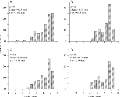
The basalar muscle is a parallel-fibered muscle whose fibers run basically in a dorso-ventral direction. The sternum, on which the fibers originate, curves upwards laterally, with the result that not all the fibers of the muscle are the same length. The fibers are longest at the medial face of the muscle and shortest at the lateral edge. The distribution of fiber lengths in the muscle was measured to determine the mean fiber length so that muscle strain during length changes imposed upon the muscle might be properly evaluated. Basalar muscles from four animals were teased apart into individual fibers whose lengths were measured with an ocular micrometer. The muscles analyzed were composed of 84–94 fibers whose measured lengths ranged from less than 4 to more than 7 mm (Fig. 1). We measured the lengths of muscles used in experiments along the medial surface, which is where the fibers are longest. In the four muscles of Fig. 1, the ratio of the mean fiber length to the muscle length measured along the medial surface was 88.2±1.4 % (mean ±S.D.). Thus, the muscle length measured along the medial surface overestimates the mean fiber length in the muscle, and underestimates the mean strain experienced by all fibers, by approximately 13 %. The muscle length used in

calculations of muscle cross-sectional area and strain are based on the mean fiber length, determined by multiplying the measured length of the muscle along its medial surface by 0.88.

Basic muscle physiology Motor unit composition of the muscle

Information on the number of motor units making up the basalar muscle was obtained by stimulating the muscle with shocks of varied intensity so as to activate differing numbers of motor units. A sudden jump in the amplitude of evoked twitches during a series of trials in which stimulus intensity was gradually increased was taken as indicating that a new motor unit had been activated; a sudden drop in twitch amplitude during a series with decreasing stimulus intensity was interpreted as indicating that the stimulus had dropped below the threshold of a previously participating unit. The stimuli were 0.2 or 1 ms voltage pulses, delivered to the muscle through implanted wire electrodes or, in some preparations, through a suction electrode on the motor nerve to the muscle. The intertrial interval ranged from 30 to 120 s in different experiments. Stimulating the basalar nerve directly lessened the possibility that the recorded responses were due in part to contraction of neighboring muscles activated by volume conduction from the implanted electrode wires, rather than responses of the basalar itself. However, the extensive dissection required to expose the basalar nerve, which destroyed some of the tracheal air supply to the muscle and

Number of

f

ibers

0 10 20

30 N=94

Mean= 6.23 mm

S.D.= 1.02 mm

0 10 20

30 N=91

Mean= 6.17 mm

S.D.= 0.85 mm

Length (mm)

1 2 3 4 5 6 7 8 0

10 20

30 N=84

Mean= 6.19 mm

S.D.= 0.96 mm

Length (mm)

1 2 3 4 5 6 7 8 0

10 20

30 N=85

Mean= 6.19 mm

S.D.= 0.91 mm

A

B

C

D

probably also interfered with the circulation of hemolymph to the muscle, apparently diminished muscle performance, and twitch forces were smaller when using nerve stimulation than with direct stimulation through implanted wires. It should be noted that ‘direct’ stimulation of an insect muscle actually activates fibers of the muscle indirectly, by exciting the motor neuron processes that course through the muscle, and motor units appear and disappear in an all-or-nothing fashion with changes in stimulus strength when using direct muscle stimulation just as they do with nerve stimulation (see, for example, Josephson, 1973).

Up to five excitatory motor units were identifiable on the basis of changing twitch amplitude with changing stimulus intensity when using either nerve stimulation or direct stimulation. Of the eight preparations in which the muscle was stimulated directly, four had five identifiable excitatory motor units, three had four excitatory units, and one had three detectable motor units. An example of the results from a preparation with five discernible excitatory motor units is shown in Fig. 2. Of the five preparations in which nerve stimulation was used, one was found to have five excitatory motor units, one had four, two had three and one had two motor units. Evidence for inhibitory innervation to the basalar muscle was found in the experiments with nerve stimulation. In five of the six preparations with nerve stimulation, in all of which the stimuli used were of progressively decreasing strength, reducing the stimulus intensity in some part of the effective range resulted in an increase rather than a decrease in twitch amplitude. The increase in twitch size with decreasing stimulus intensity suggests that the stimulus had dropped below the threshold of an inhibitory axon. The increase in twitch force associated with the dropping out of the inhibitor was approximately 20 % (21.9±3.8 %, mean ± S.D.) in the three preparations with nerve stimulation in which twitch traces were stored for later analysis. There was no evidence in these experiments for inhibitory axons when using direct muscle stimulation, although in other experiments with direct stimulation we have seen several instances of a decrease in contractile force with increasing stimulus intensity, suggesting the activation of an inhibitory axon.

The approach used above to determine the motor unit

composition of the basalar muscle gives a minimum estimate of the number of motor units in the muscle. Units that produced a very small twitch force would not be detected. Two or more units that had very similar thresholds might easily be counted as a single one. Our conclusion is that there are at least five excitatory motor axons to the basalar muscle and at least one inhibitor. These results are in broad agreement with those of Darwin and Pringle (1959), who reported 7–9 axons, presumably motor axons, in the basalar nerve of two beetle species, and with the results of Ikeda and Boettiger (1965b) who, in a detailed electrophysiological study, found eight excitatory and at least one inhibitory axon innervating the basalar muscle of a rhinoceros beetle (Oryctes rhinoceros).

Twitch and tetanic tension

The length of the muscle was adjusted to approximate the normal in vivo length as judged by the positions of the cuticular cap and apodeme of the muscle relative to surrounding structures. Twitch and tetanic responses were initiated using stimuli that were strong enough to evoke maximal contractions. The stimulation frequency for tetanic contractions was 100 Hz at 30 °C and 150–200 Hz at higher temperatures. As seems to be characteristic of asynchronous muscles, active force (the increase in force above passive level upon stimulation) is low and twitches are slow (Fig. 3; Table 1; for examples of twitch and tetanic force from other asynchronous muscles, see Machin and Pringle, 1959; Ikeda and Boettiger, 1965a; Josephson and Young, 1981; Josephson and Ellington, 1997). A temperature change from 30 to 40 °C, which is over the range at which the muscle normally operates, had surprisingly little effect on muscle contraction kinetics (Fig. 3B; Table 1). Twitch rise time shortened slightly, but not significantly (P>0.3, two-tailed t-test on paired samples), with the 10 °C increase in temperature, twitch relaxation time decreased proportionally slightly more (P<0.02), and there was essentially no change in the maximum tetanic tension. In this set of experiments, the maximum tetanic stress averaged slightly less than 20 kN m−2 _{at both 30 and}

40 °C. The measured tetanic stress was approximately twice as great in another set of experiments in which tetanic force was measured at 35 °C and at the muscle length that was optimal for work output (see Fig. 18). Why there was a large difference in

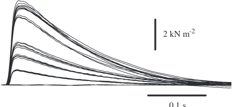
2 kN m-2

0.1 s

Fig. 2. Isometric twitches in response to repeated stimuli of progressively decreasing amplitude at 30 °C. The presence of five more-or-less discrete force levels indicates that the muscle is composed of at least five motor units.

Table 1. Some features of isometric twitches and tetanic

contractions from the beetle basalar muscle

30°C 40°C Q10

Twitch

Tension (kN m−2_{) 4.2±1.9 2.9±1.2 0.7±0.1}

Rise time (ms) 20.1±4.3 17.4±4.1 1.2±0.4

Time from peak to 50 % 105±14 68±21 1.7±0.6

relaxation (ms)

Tetanic tension (kN m−2_{) 19.1±8.0 19.2±4.5 1.1±0.4}

Twitch tension/tetanic tension 0.19±0.05 0.14±0.06 0.7±0.1

the measured stress between these two sets of measurements is not known.

Force and work at different muscle lengths

A muscle was stretched in a series of steps, beginning at a length short enough that there was little or no active or passive force. The individual length steps were 0.064 mm (approximately 1 % of muscle length). The muscle was left at each step length for 2 min. One minute after each stretch, the muscle was stimulated with a single stimulus to produce a twitch. Two minutes after the stretch, just before the next stretch, the muscle was stimulated with a tetanic burst at 120 Hz to initiate an isometric tetanus. The twitch and tetanic stimuli were adequate to produce maximal mechanical responses. During the plateau of the tetanic contraction, the muscle was subjected to a short burst of sinusoidal strain at

60 Hz with predicted peak-to-peak amplitude of 2.5–3 % (the actual strain depended on the in vivo muscle length, information about which was not available until after the end of the experiment). The sequence of stretch, twitch stimulation, tetanic stimulation and sinusoidal strain was continued as the active tetanic force rose to a maximum and began to decline. When the active tetanic force had declined to approximately 80 % of its maximum, stretching was ended and the muscle was instead shortened in a series of steps, each approximately 2 % of the in vivo length, and subjected to the same regime of twitch stimulation, tetanic stimulation and imposed cyclic strain as during the increasing length series. The muscle temperature was maintained at 35 °C throughout these experiments. The work done during the imposed cyclic strain was taken as the mean area of the work loops for cycles 2, 5 and 8 of each series. The strain amplitude used, 2.5–3 %, was well below that

Time (ms)

0 200 400 600 800 1000

S

tress (k

N

m

-2

)

0 2 4 6 8 10 12

Time (ms)

0 200 400

Relative force

0 0.2 0.4 0.6 0.8 1.0

30°C

40° C

A

B

Fig. 3. (A) A twitch and a tetanic contraction from a basalar muscle at 35 °C; tetanic stimulation frequency 150 Hz. (B) Twitches from a different basalar muscle at 30 °C and 40 °C.

95 100 105 110 115

Active force or work (% maximum) ₀ 20 40 60 80 100

Tetanus

Twitch

Wor k

Length (%L_opt)

95 100 105 110 115

Forc

e (k

N

m

)

-2

0 25 50 75 100 125

Passive Tetanic, total

A

_B

Fig. 4. Isometric force and net work at different muscle lengths during progressive muscle stretch and release. (A) Passive force and peak tetanic force (passive force plus active force). Filled symbols were obtained at progressively longer lengths during stretch, open symbols at progressively shorter lengths during the subsequent release. Two work loops, obtained with 2.8 % peak-to-peak strain, are shown. The left-hand work loop centers at the optimal muscle length, Lopt, for work output. (B) Active force (the increase in force above passive level) during twitch

optimal for work output (approximately 5.4 % at 60 Hz and 35 °C; see Fig. 10). Using a relatively small strain meant that the work output could be more accurately associated with a particular muscle length than would be true with a larger strain, one perhaps closer to the optimum and giving greater work output, but during which the muscle length would cover a greater span.

The five replicate experiments in this series all gave results similar to those illustrated in Fig. 4. The principal conclusions that we draw from these experiments are the following.

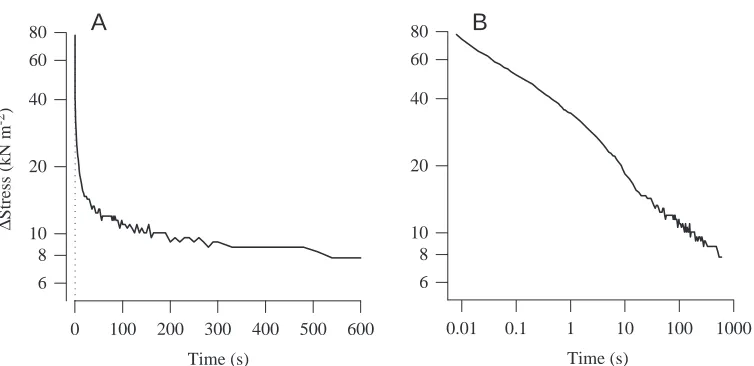
(i) Passive force during lengthening rises to a yield point, beyond which it continues to rise but at a much reduced slope (Fig. 4A). A similar yield during low-frequency stretch of passive muscle has been found in asynchronous flight muscle of the bug Lethocerus (White, 1983; Granzier and Wang, 1993a,b) and a bumblebee Bombus terrestris (Josephson and Ellington, 1997), and may be a common feature of asynchronous muscles. In synchronous muscle, force yield during stretch is commonly seen in stimulated muscle (for a review, see Josephson and Stokes, 1999), but does not seem to be a property of passive muscle (Granzier and Wang, 1993b). (ii) The effects of stretch are not reversible, at least not for stretches of the trajectory and time course used in these experiments. The muscle showed marked hysteresis during a stretch/release cycle. Passive force, active force and work were all much less for the measurements made during the progressive release following lengthening (open symbols in Fig. 4) than they were at the same muscle lengths during the preceding stretch series. Similar hysteresis has been described in other muscles, including asynchronous flight muscle from the bug Lethocerus and mammalian cardiac muscle (White, 1983; Granzier and Wang, 1993a; Granzier and Irving, 1995), where it has been ascribed to the unfolding of titin or minititin molecules during stretch (Granzier and Wang, 1993a; Helmes et al., 1999). Some of the hysteresis during a long, slow lengthening–shortening cycle of the beetle muscle may be due to length-dependent unfolding of titin or other large molecules, but some of the hysteresis is due to time-dependent processes, as is evident from the slow decline in tension (=stress

relaxation) seen after rapid stretch when the muscle is held at the stretched length (Fig. 5). Stress relaxation of stretched, unstimulated muscle, similar to that in the beetle muscle, has been described for frog (Rana esculenta, R. temporaria) muscle fibers (Buchthal et al., 1951), for the synchronous flight muscle of a locust (Schistocerca americana) (Malamud, 1989) and for the asynchronous flight muscle of a bumblebee (Josephson and Ellington, 1997). An important consequence of stress-relaxation is that muscle force during progressive lengthening, and the amplitude and shape of a length/tension curve based on measurements of muscle force, vary with the time after stretch at which the measurements are made.

C-filaments, composed of minititin, connect the ends of the thick filaments to the Z-disks of asynchronous muscles and are major contributors to the passive tension in a muscle when it is stretched (Granzier and Wang, 1993a,b). It is easy to see how non-reversible or slowly reversible unfolding of C-filaments during stretch might increase the filament compliance and lead to a substantial drop in passive tension during subsequent muscle shortening, but it is less obvious why lengthening of elements lying effectively in parallel with the thin filaments should result in a marked reduction in active tension at subsequently shortened lengths. If the C-filaments were in series with the sarcomeres, it could be proposed that their stretching allowed the sarcomeres to shorten to less favorable lengths for force production; but they are not. The depressed active force seen in the beetle muscle during the progressive shortening following stretch is consistent with the proposal of Granzier and Wang (1993a) that the amplitude of the active force produced when an asynchronous muscle is stimulated is dependent upon the passive force at the time of stimulation, and a reduction in the passive force because of C-filament unfolding leads to an associated reduction in active force.

(iii) The optimal muscle length for work output was shorter than that for isometric force (Fig. 4B). The optimal muscle length for twitch force was 2.0±0.3 % (mean ±S.E.M., N=5) greater than that for work per cycle. The optimal length for tetanic force was difficult to determine precisely because of the asymmetrical shape and broad plateau of the relationship

Time (s)

0 100 200 300 400 500 600

∆

Stress (kN m

-2)

6 8 20 40 60 80

10

Time (s)

0.01 0.1 1 10 100 1000

6 8 20 40 60 80

10

A

B

between tetanic force and muscle length; however, from inspection, it was obvious that the optimal length for tetanic force was at least as long as that for twitch force.

(iv) The length/work curves in this series were significantly narrower than the length/tension curves for twitches, which were in turn narrower than the length/tension curves for tetanic contractions. The width of the curve relating work output and muscle length, measured at 80 % of the maximum value, was 2.2±0.6 % of the optimal length (mean ±S.D., mean span was from −0.9 % of the optimal length to 1.3 %, N=5). The width at 80 % for the twitch force curve was 7.4±5.6 % of the optimal length for work output (mean ±S.D., mean span 0.6–8.0 %) and that for the tetanic force curve was 14.2±3.9 % (mean ±S.D., mean span 0.2–34.6 %).

(v) Work loops coursed in a ‘northeast’ to ‘southwest’ direction and crossed the length/tension curve for total tetanic force such that the maximum force reached during the cyclic strain of a work loop was greater than that of an isometric contraction at the maximum length reached in the loop. The position of the work loops with respect to the isometric length/tension curve was similar to that found recently for the asynchronous flight muscle of a bumblebee (Josephson, 1997a) and different from that in early reports of Boettiger (1957, 1960) and Machin and Pringle (1959), who describe work loops in asynchronous bumblebee and beetle muscles as lying entirely below the active length/tension curve or as crossing the length/tension curve but being rotated clockwise with respect to it so that the peak force in the work loop was less than that at the equivalent length in an isometric contraction.

Stretch activation and shortening deactivation

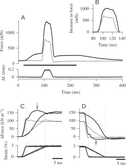
The features of asynchronous muscle that can lead to oscillatory contraction when a muscle is attached to an appropriate mechanically resonant load are delayed activation following stretch and delayed deactivation following shortening (see discussion in Josephson et al., 2000). Examples of stretch activation and shortening deactivation are shown in Fig. 6. In the experiments of this series, a muscle was stretched for a short distance at constant velocity and, after a delay, released at constant velocity. The stretch and release velocities ranged up to 75 mm s−1_{. In an unstimulated muscle, the force}

rose during stretch but then began to decline immediately at the end of stretch (Fig. 6A,C). This is the behavior expected for a passive visco-elastic structure. In a stimulated muscle, in contrast, force rose during the stretch but, at least with moderately fast stretches, continued to rise at the end of stretch to a maximum reached well after the end of lengthening. For example, in the more rapid stretch of the two illustrated in Fig. 6C, the force in the stimulated muscle reached a maximum (marked by the arrow) approximately 8 ms after the end of stretch. The increase in force following the end of lengthening is a manifestation of delayed stretch activation. With the slower stretch in Fig. 6C, some of the activation occurred during the course of the stretch, and the post-stretch rise in force, while present, is less conspicuous than that with the faster stretch. The converse of stretch activation is shortening

deactivation. The force in an unstimulated muscle, as expected for a passive element, fell steadily during shortening and remained more-or-less constant after the end of shortening (Fig. 6D). In a stimulated muscle, the force dropped rapidly during shortening, but then continued to drop to a minimum reached well after the end of shortening. The continued drop in force after shortening reflects delayed deactivation.

Figs 4 and 6 also illustrate another feature that is apparently common to asynchronous muscles, high resting stiffness (see discussion in Josephson et al., 2000). Synchronous muscles,

Time (ms)

0 100 200 300 400

∆

L

(mm)

0 0.2

Force (mN)

0 500 1000

Time (ms) 80 100 120 140

Increase in force

(mN)

0 500 1000

A

B

∆

Force (kN m

-2)

0 50 100 150

Strain (%) 0 3

0 50 100 150

0 3

5 ms 5 ms

C

D

Fig. 6. Force changes in a beetle muscle during ramp stretch and release. Force and length (L) traces for the unstimulated muscle are shown as thin lines, those from the tetanically stimulated muscle are the thicker lines. (A) Stretch and release imposed on a muscle when unstimulated and during tetanic stimulation. The total length change was 0.185 mm, and the stretch and release velocity was 15 mm s−1_.

The time of muscle stimulation (1 ms pulses at 100 Hz) is marked by the horizontal bar beneath the force traces. (B) The increase in force above the pre-stretch level during the stretch and release. (C) Muscle force during stretch, on an expanded time scale, for stretches at 15 mm s−1_{and at 75 mm s}−1_{. The dotted vertical lines mark the end of}

the fast and slow stretches. The arrow indicates the time of peak force during the delayed activation following the fast stretch. (D) Decrease in force during shortening at 15 mm s−1 _{and at}

75 mm s−1_{. The dotted vertical lines mark the end of the fast and slow}

such as vertebrate skeletal muscles, are relatively compliant when unstimulated and become stiff, resistant to stretch, when stimulated. The beetle muscle is rather different from synchronous muscles in that its stiffness, as judged by the trajectory of the force increase early in stretch, is similar in passive and in active muscle. With the short, fast stretches of Fig. 6C, the force rise is nearly identical in the stimulated and in the unstimulated muscle, indicating similar stiffness in the two. With the slower stretch of Fig. 6C, the force rise is initially similar in the stimulated and unstimulated muscle, but the force trajectories diverge later, with the force rising more rapidly in the stimulated muscle. It seems likely that some, if not all, of the separation of the force trajectories of the unstimulated and stimulated muscle is a result of delayed stretch activation in the latter.

Muscle activation during tethered flight

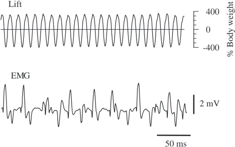
Muscle action potentials were recorded from a basalar muscle in animals that flew while attached to a force transducer by the dorsal pronotum. The transducer measured the force resulting from wing movements. The basalar muscle has a number of motor units (see above), and the electrical recordings were often rather complex. An experiment was deemed successful if the animal flew and if there was at least one motor unit whose electrical signals were large and repeatedly identifiable in the electrical recording. In the first five successful experiments, the animal was linked to the transducer by way of an insect pin mounted perpendicularly to the transducer blade. The force records in these animals included components of both lift and thrust. In a subsequent set of experiments, five of which were rated as successful, the force recording was improved by mounting the animal directly to the transducer blade such that the force signal represented lift alone (Fig. 7). Values for the frequency of wing strokes and muscle action potentials are based on analysis of five segments, each 0.5–1 s in duration, from each animal.

The wing-stroke frequency recorded from animals in tethered flight was 77.6±9.2 Hz (mean ± S.D., N=10 animals). Measurements of electromyographic (EMG) frequency were made from the motor unit with the largest electrical signal. The firing frequency of the largest unit averaged 21.1±12.0 Hz (mean ±S.D., N=10 animals). While it seems likely that the EMG spikes that we measured were from a single unit in each preparation, it is possible that in some preparations there were two or more motor units producing spikes of similar large size that were counted together, which would make the measured frequency an overestimate of the firing frequency of a single motor unit. As is characteristic of asynchronous muscles, there are many oscillatory muscle contractions for each electrical event.

The lift generated by the wing strokes went through large, nearly sinusoidal oscillations about the zero line. The maximum upward and downward forces were both over three times the animal’s body weight (Fig. 7). An average lift of 100 % of body weight would be required to keep the animal airborne in free flight. In tethered animals, the lift averaged over many cycles was only approximately 20 % of body weight (19.8±9.4 %, mean ±S.D., N=5 animals). The power output of the tethered animals was substantially less than that required to keep them airborne in free flight.

The determinants of power output

The obvious variables affecting mechanical power output by an asynchronous muscle are muscle length, strain amplitude, strain trajectory (i.e. sinusoidal, sawtooth, symmetrical or asymmetrical, etc.), cycle frequency, muscle temperature and the degree of muscle activation which, in living muscles, is presumably determined by the frequency of activating stimuli (in a synchronous muscle, the degree of muscle activation would be replaced as a variable by the pattern and phase of activation in the strain cycle). The following considers the effects of changes in most of these variables on work and power output. To make the task of evaluating the determinants of work output more manageable, we used sinusoidal strain throughout and have not considered the effects of strain trajectory.

The method for measuring work output

The usual approach used to quantify the effects of changes in a selected variable on mechanical work output is illustrated in Fig. 8. A basalar muscle was stimulated tetanically and subjected to a series of sinusoidal length changes (=strain) imposed during the plateau of the tetanic contraction. The control signals to the ergometer that produced the length changes were generated by a computer. In most experiments, the sinusoidal amplitude, the frequency or the muscle length at mid-cycle was changed by a predetermined amount after every third cycle. Thus, the sinusoidal waveform consisted of a continuous series of three-cycle sets, with a progressive change in the value of one variable between sets. In Fig. 8, it is the strain amplitude that was altered between sets. A single trial, such as that illustrated in Fig. 8A, consisted of 6–8 sets, and thus 18–24 sinusoidal cycles. Varying the value of a variable

Fig. 7. Lift generated by wing strokes (upper trace) and muscle action potentials recorded from a basalar muscle (EMG; lower trace) during tethered flight. The horizontal line through the lift trace is zero lift, i.e. the force on the transducer when the beetle hung passively from it.

EMG Lift

% Body weight

-400 0 400

2 mV

during a trial gave us multiple determinations of the effects of that variable during a single trial. A variable that was changed progressively within a single trial will be referred to as a within-trial variable, as opposed to a between-trial variable, which was altered between trials. Values of muscle length and force during a trial were collected by a computer (sampling rate 15 kHz). A computer program, written in LabVIEW (National Instruments Corp, Austin, TX, USA), generated the sinusoidal control signals, identified the second cycle in each set, displayed this cycle as a work loop (Fig. 8C), and calculated and displayed relevant features of the loop (maximum and minimum muscle length, maximum and minimum force, cycle frequency, work done). The program, designed for measuring work from asynchronous and synchronous muscles, is available from the authors by request. This program requires a PC computer, LabVIEW 5.0 and an appropriate A/D board.

Experimental trials in which there was tetanic stimulation were spaced regularly at 2 min intervals. Several pacing trials, in which the muscle was stimulated tetanically while held at constant length, preceded the series of trials in which data on work performance were collected. Occasionally, trials without stimulation, intended to evaluate the mechanical properties of a passive muscle, were interposed in the interval between trials with stimulation. Muscles were moistened periodically with locust saline throughout an experiment. The thoracic temperature in all experiments was maintained at 35 °C unless stated otherwise.

Each experiment began with a determination of the stimulus intensity needed to activate the muscle fully and, in most experiments, an evaluation of the optimal muscle length and strain for work output. The appropriate stimulus intensity was determined by stimulating the muscle with a brief tetanic burst (1 ms shocks at 100 Hz, 150 ms burst duration). The stimulus

3 5 1

Strain (%)

-2 0 2 4

Force (kN m

-2)

0 100 200

3 5 1

Total strain (%) 2 4 6 8

Work (J kg

-1)

0 1 2

100 kN m-2

50 ms 5%

100 kN m-2

50 ms

5%

A

B

C

D

intensity, which was initially subthreshold, was doubled from trial to trial (intertrial interval 1 min) until the evoked isometric contraction reached a maximum. The stimulus intensity used in experiments was twice the minimal intensity needed to produce a maximal response. The procedure used to identify an appropriate muscle length and strain was as follows. The muscle was set initially at a length judged visually to be slightly shorter than the in vivo length. The muscle was then stimulated tetanically and, during the plateau of the tetanic contraction, subjected to a burst of sinusoidal strain, usually at 60 Hz. The initial strain amplitude was chosen to be close to the expected optimal value, on the basis of the animal’s size. The muscle length was increased after every third cycle of the strain series, typically by 0.02 mm (approximately 0.3 % of muscle length). The muscle length was then set at the length that had given the greatest work in this series. Next, the optimal strain was determined as in Fig. 8. The muscle was stimulated tetanically and subjected to 60 Hz sinusoidal strain, the amplitude of which was increased progressively through the burst. If the strain that gave the greatest work output was found to be significantly different from the initial, estimated value for optimal strain, the optimal length was redetermined using the new value for optimal strain. Trials in which length was varied alternated with those in which strain was varied until optimal values for both variables were established.

The relationship between work output per cycle and either muscle length or the amplitude of imposed strain was an inverted U-shaped function (e.g. Fig. 8D), as was the relationship between power output and cycle frequency. The optimal value of the independent variable (length, strain or frequency) in trials giving results such as that in Fig. 8D was determined by fitting a second-order polynomial to the data using the analysis routine in the plotting program SigmaPlot (SPSS, Inc., Chicago, IL, USA). The second-order polynomial was differentiated, the differential was set equal to zero, and the resulting equation was solved to obtain the optimal value of the independent variable. The optimal value of the relevant variable was substituted back into the original second-order polynomial to obtain the maximum work or power output, that at the optimal value of the independent variable. As a check on this procedure, the maximum power output predicted by curve-fitting in one set of experiments was compared with the maximum power output actually recorded. The experiments used in this comparison were those in which maximum power at the wing-stroke frequency and thoracic temperature of free flight was determined as a function of muscle strain (see below). The mean maximum power predicted by curve-fitting in 12 preparations was 125 W kg−1_{, the mean of the maximum}

power actually measured in the 12 preparations was 127 W kg−1_{. The difference between the maximum measured}

power and the predicted maximum power was +1.9±3.3 % (mean ±S.D.). Determining maximum work or power by fitting a polynomial to the recorded data does not introduce a significant error. It is not surprising that the measured maximum values are slightly greater than those predicted by curve-fitting. Because of experimental noise, some data points

are expected to lie below and some above a fitted curve, and the largest of the measured points is likely to be one of those above the curve.

In many experiments, the principal between-trial variable was presented in either an increasing or a decreasing series, followed by a mirror series in the reverse order. For example, in the next set of experiments to be considered, the between-trial variable was cycle frequency. In half of these experiments, optimal muscle strain (the within-trial variable) was determined in a series of trials at increasing cycle frequency, followed by a second, similar series of trials at decreasing cycle frequency. In the other half of the experiments, the first series was of decreasing frequency and the second of increasing frequency. In these experiments, each series took approximately 30 min to complete. There was some deterioration in the preparations over the course of an experiment and, in all cases, no matter what the between-trial variable, the maximum work per cycle was consistently less in a second series than in the first. In the experiments in which cycle frequency was the between-trial variable, the mean reduction in the maximum work per cycle between the first and second series was 24 % (range 12–38 %). Since the two series were not equivalent, at least for work output, it seemed inappropriate to combine them as we had intended to do when planning the experiments. Therefore, in these experiments, and in similar experiments involving other between-trial variables, the results to be reported are from the first series alone.

Work output as a function of strain and cycle frequency

Optimal muscle strain was evaluated at cycle frequencies of 30, 40, 50, 60, 80 and 100 Hz. The muscle length throughout was that determined to be optimal at 60 Hz. The muscle was

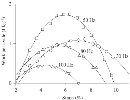
Fig. 9. The relationship between the amplitude of imposed strain and the work done per cycle, measured at different cycle frequencies. The symbols are individual data points, and the continuous lines are second-order polynomials fitted to these points. The optimal strain was obtained by differentiating the second-order polynomial, setting the resulting differential to zero, and solving the equation. Results obtained with cycle frequencies of 40 and 60 Hz in this experiment have been omitted for clarity.

Strain (%)

2 4 6 8 10

Work per cycle (J kg

-1)

0 1 2

100 Hz

80 Hz 50 Hz

subjected to two sets of strains with interleaved values at each frequency (see Fig. 8D). Six animals were used in these experiments. In three preparations, the first frequency used was 30 Hz, and the frequencies were progressively increased through the series; in the other three preparations, the frequencies were presented in descending order.

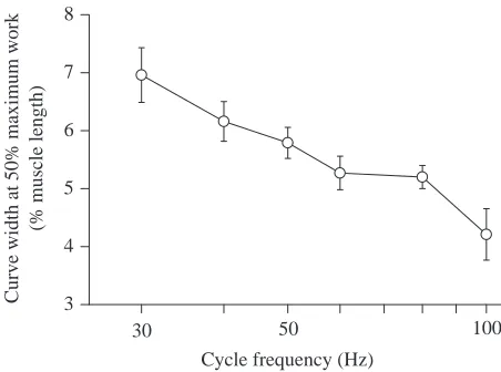
The work output per cycle was strongly dependent on strain, and there was an obvious optimal strain at each cycle frequency examined (Fig. 9). The optimal strain declined progressively as the cycle frequency increased, falling from approximately 7 % at 30 Hz to 4 % at 100 Hz (Fig. 10). The width of work versus strain curves also declined progressively with increasing cycle frequency (Fig. 11). The work per cycle at the optimal strain was greatest at the 50 Hz cycle frequency

(Fig. 12). Mechanical power output, which is the product of work per cycle and cycle frequency, rose with increasing cycle frequency to reach a maximum at 60–80 Hz, and declined when the frequency was increased further to 100 Hz (Fig. 12).

The usual inverse relationship between muscle force and shortening velocity dictates that there is an optimal shortening velocity for mechanical power output. If a muscle is to operate at or near this optimal velocity while shortening, there should be an inverse relationship between the cycle frequency and the strain per cycle. There is a decrease in optimal strain with increasing cycle frequency in the beetle muscle, but the decline in optimal strain with increasing cycle frequency is not great enough to result in the muscle operating at a single, optimal shortening velocity across the frequency range examined. The maximal velocity reached during a sinusoidal length trajectory and the mean velocity during the shortening portion of the cycle are both proportional to the product of strain and cycle frequency, and both measures of velocity increase with increasing cycle frequency for muscle operating at the optimal strain (Fig. 10).

Work output as function of muscle length

In this group of experiments, the within-trial variable was muscle length. The length was initially set well below that anticipated to be optimal for work output, and the length was increased from set to set throughout the trial in steps that were great enough that the length passed through and beyond the optimum. The relationship between muscle length and work output was determined at a series of strains, ranging from approximately 2 to 10 %, and at cycle frequencies of 40, 60 and 90 Hz. This experiment was repeated with four preparations, each of which gave basically similar results leading to the following conclusions.

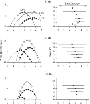
(i) At normal operating frequencies, the work output is positive over only a very limited range of muscle length (Fig. 13). In the experiment shown in Fig. 13, the maximum work per cycle occurred at the 60 Hz cycle frequency and with

Cycle frequency (Hz)

Optimal strain (%)

3 4 5 6 7 8

30 50 100

0 5 10 15

Velocity (lengths s

-1)

Average velocity

Maximum velocity

Strain

Fig. 10. Optimal strain (filled symbols, means ± 2 S.E.M., N=6) and shortening velocities at the optimal strain (open symbols) at different cycle frequencies. Maximum velocity (=πFS, where F is cycle frequency and S is peak-to-peak strain) is indicated by circles, and mean velocity during shortening (=2FS) is indicated by squares.

Fig. 11. The width of work versus strain curves, such as those of Fig. 9, at different cycle frequencies. The width of each curve was measured at 50 % of the maximum work for that curve. Values are means ± 2 S.E.M., N=6.

Cycle frequency (Hz)

Curve width at 50% maximum work

(% muscle length)

3 4 5 6 7 8

30 50 100

Frequency (Hz)

Maximum work per cycle (J kg

-1)

0 1 2

0 25 50 75 100

30 50 100

Work

Power Power (W kg

-1)

muscle strain of 4.2 %. The curve of work output versus muscle length for these values of frequency and strain in Fig. 13 (left-hand column, middle panel, open circles) has a width measured at half-maximal work of only 2.9 %. In the three other experiments of this series, the width, measured similarly, of that work versus length curve with the greatest maximum work at 60 Hz was 2.7 or 2.8 %.

(ii) The work versus muscle length curves become increasingly narrow as cycle frequency is increased (Fig. 13). The mean width of the curves with the greatest peak work, again measured at half-maximal work, was 4.9 % (range 3.9–6.5 %) at 40 Hz, 2.8 % (range 2.7–2.9 %) at 60 Hz and 2.7 % (range 2.4–2.9 %) at 90 Hz.

(iii) The optimal length for work output declines as strain is increased (Figs 13, 14). The change in optimal muscle length with increasing strain is such that, if the muscle is at optimal length at mid-cycle, the maximal length reached during stretch increases little with increasing strain, while the minimal length reached during shortening declines substantially.

-3 -2 -1 0 1 2 3

Work (

µ

J per cycle)

0 1 2

-3 -2 -1 0 1 2 3

0 1 2

40 Hz

Muscle length (% change from reference length)

-3 -2 -1 0 1 2 3

0 1 2

-6 -4 -2 0 2 4

Strain (%)

0 2 4 6 8 10

-6 -4 -2 0 2 4

0 2 4 6 8 10

-6 -4 -2 0 2 4

0 2 4 6 8 10

60 Hz

90 Hz

Length range

Lopt

2.7% 4.2% 7.8%

Fig. 13. The relationship between muscle length and the work done per cycle, measured at different muscle strain and cycle frequency. The reference length used in the abscissa of all panels was that length found to be optimal for work output at 60 Hz in the set-up trials before the main experiment. Left-hand panels: work output as a function of muscle length at three different strains. These results are from an experiment in which muscle length was changed progressively during a trial. In each panel, the results from a single trial are shown by a common symbol. The continuous lines are second-order least-squares regressions fitted to the results of a trial. The numbers above the data sets in the upper left-hand panel show the peak-to-peak strain for that data set and for the data sets with the same symbol in the two panels below. Some sets of data were obtained at different strain levels from those shown but, to increase the clarity of the presentation, they have not been plotted. The three panels show results obtained at cycle frequencies of 40, 60 and 90 Hz as indicated. Right-hand panels: optimum muscle length for work output (Lopt, filled symbols) and the length changes

experienced by a muscle during sinusoidal strain cycles when operating at the optimum length for different strains and cycle frequencies (horizontal lines). The optimal muscle lengths were obtained by differentiating the second-order polynomials shown as continuous curves in the left-hand panels, setting the resulting differentials to zero, and solving the equations.

Fig. 14. Change in optimal muscle length with increasing strain, relative to that at the smallest strain tested; cycle frequency 60 Hz, temperature 35 °C. Each set of symbols joined by a line is from a single preparation. Data shown by the filled symbols are from the same preparation as in Fig. 13. The diagonal broken lines have a slope of −1/2 and are given for reference. The maximum muscle length reached in a cycle is the initial length plus half the peak-to-peak strain. For the maximum muscle length reached in a cycle to remain constant, the initial muscle length should decrease with increasing strain by an amount equal to half the strain; i.e. with the

slope shown by the broken lines. Strain (%)

0 2 4 6 8 10

Change in optimal length (% muscle length)

Optimal cycle frequency and power output at different temperatures

In these experiments, cycle frequency was the within-trial variable and temperature was the between-trial variable. To increase resolution, pairs of trials, the second of which had values that interdigitated with the first, were given at each temperature. The muscle length and strain amplitude were those found to be optimal for work output in a series of test trials at 30 °C and a cycle frequency of 50 Hz. The test trials immediately preceded the experimental trials in which cycle frequency and temperature were varied. The temperatures used were 25, 30, 35 and 40 °C. In three preparations, the temperatures were presented in increasing order, in three preparations in decreasing order.

The optimal cycle frequency and the power output at that frequency increased in parallel with increasing muscle temperature (Figs 15, 16). The limits of the frequency range over which there was positive power output were not explored, but it was clear that the curves relating cycle frequency and power output were rather broad, with positive power over at least a fourfold range of frequencies. The peak power output in these experiments, that at 40 °C and 60–70 Hz cycle frequency, was slightly greater than 100 W kg−1

(104±24 W kg−1_{, mean ±S.D.).}

Optimal strain, work per cycle and power output at different temperatures

The following experiments were performed to characterize better the effects of temperature on work output by the muscle. The within-trial variable was strain; the between-trial variables were cycle frequency (40, 60 and 90 Hz) and temperature (25–40 °C in steps of 5 °C). In three preparations, the three cycle frequencies were presented during each of a set of

increasing temperatures; in three preparations, the temperatures series was decreasing.

At least in synchronous muscles, shortening velocity is strongly dependent on temperature, with Q10 values for

maximum shortening velocity typically being 1.5–3 in the normal range of operating temperatures (Bennett, 1984). Therefore, we anticipated that the optimal strain at a given cycle frequency would be strongly dependent on muscle temperature and that the work per cycle would increase with temperature. We reasoned that, because of a higher shortening velocity, the optimal distance of shortening during a cycle, and therefore the optimal strain, would increase with increasing temperature and that the greater strain would lead to greater work output. In fact, the optimal strain was found to be only weakly dependent on temperature (Fig. 17A). Increasing the temperature from 25 to 40 °C increased the optimal strain by only 24 %, 23 % and 40 % at cycle frequencies of 40, 60 and 90 Hz respectively. Further, although the work per cycle did increase monotonically with increasing temperature at the 90 Hz cycle frequency, at 40 and 60 Hz, the work per cycle at optimum strain passed through a maximum and then declined with further increase in temperature (Fig. 17B). There was a general tendency for the maximum power output at 40, 60 or 90 Hz to increase with temperature, but the peak power at 40 °C (94 W kg−1

with 90 Hz cycle frequency) was not significantly greater than that at 35 °C (93 W kg−1 _{with 60 Hz). The relative}

insensitivity of optimal strain to temperature change and the complex relationship between work output and temperature probably result from temperature affecting, sometimes in contradictory ways, both muscle shortening velocity and the time course of the deactivation processes that underlie asynchronous operation. We will return to this in the Discussion.

Fig. 15. The effects of changing cycle frequency on mechanical power output measured at different temperatures. The muscle length and strain were those determined to be optimal for work output at 30 °C and a cycle frequency of 60 Hz. The temperatures in this example were presented in decreasing order.

Frequency (Hz)

0 20 40 60 80 100

Power (W kg

-1)

0 20 40 60 80 100 120 140

25°C 30°C

35°C 40°C

Thoracic temperature (°C)

25 30 35 40

Optimal frequency for power (Hz)

0 10 20 30 40 50 60 70

0 25 50 75 100 125

Power at optimum frequency (W kg

-1) Frequency

Power

Fig. 16. Effects of temperature on the optimal frequency for power output and the power output at the optimal frequency. The results are from experiments such as that in Fig. 15. Values are means ± 2

S.E.M., N=6. The Q10values for the temperature range 25–40 °C were