A dataflow architecture for beamforming operations

(1)

A dataflow architecture for beamforming operations

Msc Assignment

by

Rinse Wester

Supervisors:

dr. ir. Andr´e B.J. Kokkeler dr. ir. Jan Kuper ir. Kenneth Rovers Anja Niedermeier, M.Sc

ir. Andr´e W. Gunst dr. Albert-Jan Boonstra

Computer Architecture for Embedded Systems Faculty of EEMCS

University of Twente

(2)

(3)

Abstract

As current radio telescopes get bigger and bigger, so does the demand for processing power. General purpose processors are considered infeasible for this type of processing which is why this thesis investigates the design of a dataflow architecture. This architecture is able to execute the operations which are common in radio astronomy.

The architecture presented in this thesis, the FlexCore, exploits regularities found in the mathematics on which the radio telescopes are based: FIR filters, FFTs and complex multiplications. Analysis shows that there is an overlap in these operations. The overlap is used to design the ALU of the architecture. However, this necessitates a way to handle state of the FIR filters.

The architecture is not only able to execute dataflow graphs but also uses the dataflow techniques in the implementation. All communication between modules of the architecture are based on dataflow techniques i.e. execution is triggered by the availability of data. This techniques has been implemented using the hardware description language VHDL and forms the basis for the FlexCore design. The FlexCore is implemented using the TSMC 90 nm tech-nology.

The design is done in two phases, first a design with a standard ALU is given which acts as reference design, secondly the Extended FlexCore is presented. The Extended FlexCore incorporates the ALU which exploits the regularities found in the mathematics. The ALU of the Extended FlexCore is able to perform a four point FIR filter, a complex multiplication or an FFT butterfly operation in a single clock cycle. The Extended FlexCore uses an Explicit State Store (ESS) to handle stateful operations like a four point FIR filter.

The standard FlexCore and the Extended FlexCore are compared by exe-cuting a FIR filter, FFT and complex multiplications. The comparison shows that the Extended FlexCore is significantly more energy efficient per operation than the reference FlexCore.

Finally, an indication of the energy efficiency of the Extended FlexCore is given in comparison with other architectures. It is shown that the FlexCore lies, in terms of energy per operation, between the ASICs and the general purpose ARM processor.

(4)

(5)

Introduction

A way to summarise the developments in radio astronomy is ”the bigger, the better”. Especially radio telescopes like LOFAR reach sizes over 1500 kilome-ter across[1],[2]. An even bigger telescope, SKA, is planned to be operational in 2023. SKA will have a total collecting area of 1 square kilometer and has a diameter of more than 3000 kilometer[3],[4]. All these telescopes use a huge number of antennas to receive the signals. All these signals are combined into sky pictures by a technique called beamforming.

With the increase in size and number of antennas, so does the demand for processing power to handle all the data coming from these antennas. Conven-tional processors like von Neumann architectures are considered infeasible for these types of applications in terms of processing power and energy consump-tion which is why the radio astronomy community uses ASICs and FPGAs [5],[6],[7].

In this thesis, an implementation of the dataflow architecture proposed by Kenneth Rovers [8], the FlexCore, is presented. Parts of the algorithms used in radio astronomy are used to evaluate the FlexCore to see whether dataflow architectures are suitable for applications like radio astronomy.

1.1

Research goals

The goal of this thesis is to implement the FlexCore using the hardware de-scription language VHDL. After that, the design should be synthesized using ASIC tooling such that numbers like area and power consumption can be ex-tracted. The FlexCore is a dataflow architecture where execution is triggered by the availability of data instead of a program counter (dataflow execution). The corresponding models used for analysis of execution based on availability is called dataflow analysis.

The FlexCore itself also uses data triggered execution for all the inter-nal modules of the design. The FlexCore can therefore also be considered a dataflow graph. All the connections in this graph (connections between the modules of the architecture) use buffers with feedback for communication. This feedback prevents overflows of the buffers and is called backpressure[9]. Before implementing the FlexCore, dataflow graphs with backpressure should

(8)

CHAPTER 1. INTRODUCTION 2

be implemented using VHDL first. This will form the basis on which the de-sign of the whole FlexCore is based. The corresponding research question is: How can dataflow graphs with backpressure be implemented in VHDL and what will be the lower bound of the buffer sizes?

The reason for trying to combine dataflow architectures and beamforming is that dataflow programs lie closer to the mathematical description of the program than for example von Neumann architectures. However, dataflow ar-chitectures introduce overhead due to the fine grain parallelism[10]. An impor-tant way of increasing energy efficiency is exploiting locality of reference[11]. The main research question for this thesis is: How can the granularity of dataflow execution be increased by exploiting locality of reference in the LO-FAR beamforming application?

1.2

Thesis structure

Background information is given in chapter 2 about the concepts that will be used throughout this thesis. First an introduction on dataflow graphs will be given, followed by how these are executed in dataflow architectures. Finally, more information is given on beamforming and how this is implemented on the LOFAR radio telescope.

As dataflow principles are the major part of the design of the FlexCore, they are first implemented in hardware using the hardware description lan-guage VHDL. Chapter 3 shows how dataflow graphs are implemented using VHDL and how much buffering of data is required. In order to exploit lo-cality of reference by increasing the granularity, the mathematical operations used for radio astronomy are investigated in chapter 4. Regularities in the algorithms of beamforming are used to merge the basic components of these algorithms together into a single module of the processor.

In order to evaluate these ideas, two implementations of the FlexCore are made. The first implementation, referred to as standard FlexCore, is a standard dataflow architecture as described in literature[12]. The standard FlexCore is used as reference implementation to evaluate the Extended Flex-Core which incorporates the regularities found in the beamforming applica-tion. Chapter 5 starts with the implementation of the standard FlexCore and elaborates on the techniques used to design this processor (dataflow). In section 5.3 the Extended FlexCore is presented exploiting the mathematical transformations from chapter 4.

Both designs have been implemented using 90 nm technology. Also several algorithms have been executed on both designs such that an indication of power usage can be given. The results of this can be found in chapter 6 and are compared to other architectures in chapter 7.

(9)

2

Background

Before diving into dataflow graphs, dataflow machines and beamforming, some background information about dataflow graphs, dataflow architectures and beamforming is needed. This chapter gives the background information on which the rest of this thesis is based. First a basic explanation on dataflow graphs is given in section 2.1. This is used in section 2.2 where the inner working of dataflow machines is explained. Section 2.3, gives the information on beamforming which is the application of which parts should run on the FlexCore. Finally, section 2.4, explains the tool flow for building an ASIC.

2.1

Dataflow graphs

Data Flow Graph (DFG)s are mathematical representations of programs[13]. Execution of these programs is not driven by a sequence of instructions but by the availability of data. The most well known type of dataflow graphs are Synchronous Data Flow (SDF) graphs[14]. Dataflow graphs are the basis for the work presented in this thesis.

The operations that should be performed during execution of a dataflow graph are represented bynodes. Nodes can be of any granularity, ranging from simple operations like addition and multiplication to complete FFT operations and processors. Nodes in a dataflow graph are connected by arcs which do not only represent the dependencies between nodes but which are also the locations where data is stored. The packets containing data are so called

tokens. Figure 2.1 shows the terminology displayed graphically.

x2 ₊

node arc

token

Figure 2.1: Simple dataflow graph forx2₊_x2

The execution of a dataflow node is triggered by the availability of tokens. When all required inputs for a node are available the node becomes enabled.

(10)

CHAPTER 2. BACKGROUND 4

An enabled node consumes tokens on the input(s) and produces tokens on the output(s). This process is called firing. Only enabled nodes may fire which is called the firing rule i.e. the firing rule states that a node may only execute when all required tokens are available on the input(s).

A B 3

+ n1 / n2 result (a)

A B 3

+ n1 / n2 result (b)

A B 3

+ n1 / n2 result (c)

A B 3

+ n1 / n2 result (d)

Figure 2.2: Firing rules in dataflow graphs

Figure 2.2 shows four events during execution of a dataflow graph created from the formula result = A+₃B. Node n1 (the adder) is the first to receive

a token but is not yet enabled because it requires two tokens. At a later time (figure 2.2b) the second token has arrived as well and node n1 becomes

enabled. Noden2 (the divider) also receives a token but remains disabled until

n1 has produced its result. Figure 2.2c shows the time wheren1 has produced

a result and therefore enables noden2. Whenn2 fires it consumes the tokens

on the inputs and produces a token containing the result (figure 2.2d). A graph whose nodes only consume and produce a single token per input and output during firing are called Homogeneous Synchronous Data Flow (HSDF) graphs [15]. Homogeneous dataflow graphs are a subset of Syn-chronous Data Flow (SDF) graphs[14] which can produce and consume several tokens at once. The work presented in this thesis however only involves Ho-mogeneous Synchronous Data Flow (HSDF) graphs.

The time between two events in a Synchronous Dataflow Graphs can be arbitrary. A pure implementation of such graphs therefore does not require a global clock because all the synchronization is enforced by the firing rules. More information can be found in the literature report which is included in appendix B. More theoretical information on dataflow graphs can be found in [15] and [16].

2.2

Dataflow architectures

(11)

CHAPTER 2. BACKGROUND 5

Dataflow machines are usually divided in two groups, the static dataflow machines and dynamic dataflow machines. In static dataflow machines, the DFG being executed does not change. In a dynamic dataflow machine how-ever, the DFG is able to change during execution. Dynamic dataflow machines are able to perform more advanced features like procedure calls. More infor-mation about different dataflow machines can be found in the literature report in appendix B and in [12].

The architectures presented in this thesis use principles from both static and dynamic dataflow machines. Figure 2.3 shows the general structure of a static dataflow machine. The dataflow graph is usually stored in a special memory. This memory also supports storage of tokens. As can be seen in figure 2.3 every incoming token from the left triggers the enabling unit to detect whether a node from the DFG becomes enabled. If this is not the case, the token will be stored in the memory. When a node becomes enabled, i.e. there is a match, both operands and instruction for that particular node are combined in a packet and sent to the functional unit which executes the instruction with the given operands. After the instruction has been completed, the result is sent to the enabling unit again. Resulting tokens may enable other nodes from the DFG which completes the cycle.

enabling unit

memory for tokens and nodes

functional unit

Figure 2.3: Basic structure of a static dataflow machine.

The matching procedure in static dataflow machines requires special hard-ware for every possible node in the DFG. The hardhard-ware has three registers: one for the instruction and two for the operands (the in-degree of nodes is usually two). When both operand registers contain a value, a match is found. Static dataflow machines like the MIT static dataflow machine therefore have a matching circuit for every node[17]. More information about static dataflow machines can be found in the literature report in appendix B.

(12)

CHAPTER 2. BACKGROUND 6

ETS

A more efficient way of matching instead of using hashing functions is an Explicit Token Store (ETS) which was introduced in a machine called the Monsoon[19]. The ETS was specifically designed for efficient execution of procedure calls. The central idea behind ETS is to allocate large blocks of memory for complete procedures but let the addressing details of single vari-ables in the program be determined at compile time. Both FlexCores do not support procedure calls but do make use of the addressing techniques that should be applied at compile time. Therefore this explanation will only focus on the addressing part, a complete view of the ETS can be found in literature report of appendix B.

The addressing for an ETS is performed by the compiler. Every node in the dataflow graph is assigned a unique address. This address is then used for both the instruction in the program memory and tokens that have to be stored before a match occurs. Consider the following dataflow graph.

A B

3

− n0

+ n2 /

n1

Out0 Out1

hn2.R5i

addr instr dests

0 SUB n1.R,n2.R

1 ADD out

2 DIV out

Program memory

addr p value

0 false 1 true 5 2 true 5

Token memory

Figure 2.4: Example of ETS-principle.

Figure 2.4 shows an example dataflow graph with the corresponding mem-ory contents of a dataflow machine. All nodes of the DFG are assigned a unique address that is used in both the token memory and the program mem-ory. The program memory contains the instruction that corresponds to the operation in the DFG and a set of destinations. Node n0 for example is

as-signed address 0 and has two destination nodes (right input of n1 and n2)

which use the produced result.

(13)

CHAPTER 2. BACKGROUND 7

is f alse no token is on any input so the incoming token should be stored in the token memory(see address 1 and 2). If the bit was set to true it means that the incoming token causes a match. The value of the previously stored token should then be fetched from the token store. Both the incoming token and the one from the token store form the operands for the instruction that is addressed by the incoming token. The instruction has a set of destinations to which the result is sent. These resulting tokens may enable other nodes which completes the cycle.

2.3

Beamforming

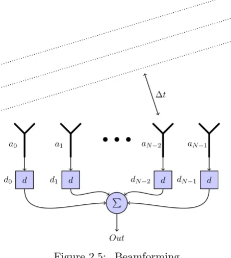
Beamforming is a technique used in radio astronomy to combine signals from several antennas. Using this technique, a much better directivity can be achieved. Signals which would normally be undetectable due to noise, can now be received if enough antennas are used. Beamforming uses the fact that the antennas are separated from each other by a certain distance. Signals from a certain angle therefore do not arrive at the same time. Adding the proper delay to the received signals makes the system directive. Figure 2.5 shows this process graphically.

a0 a1 aN−2 aN−1

∆t

d

d0 d1 d dN−2 d dN−1 d

P

[image:13.595.182.409.404.657.2]

Out

Figure 2.5: Beamforming

Figure 2.5 shows an array of N antennas which are combined with de-lays d0. . . dN−1. Signals (the wavefront shown with dashed lines) arrive first

(14)

CHAPTER 2. BACKGROUND 8

such that all received signals are in phase again, the sum of all signals has a much better signal quality than a signal from a single antenna. There are several techniques to perform beamforming[20] and to implement the delays as shown in figure 2.5. LOFAR uses frequency beamforming to implement these delays[2].

From Fourier theory it is known that a delay can be implemented by multiplying the Fourier transform of the signal with a complex phase shift (equation (2.1)). More information on Fourier theory can be found in [21],[22].

f(t₋τ) _↔ fˆ(ω)e−iωτ (2.1)

f(t) is a signal in the time domain being delayed with time τ. The time domain signal f(t) has a corresponding signal ˆf(ω) in the frequency domain.

ˆ

f(ω) =_F(f(t)) i.e. ˆf(ω) can be found by taking the Fourier transform of the time domain signalf(t). The signalf(t) is now delayed by multiplying it with a complex phase shifte−iωτ.

Delaying a signal by using a phase shift only works perfectly for sinusoid functions. However when the bandwidth of the signal f(t) is small enough, the phase shift can still be used. To determine if the bandwidth of the signal is ”small enough”, a measure called the Fractional Bandwidth (FB)[23] is used. The Fractional Bandwidth is a number that gives a comparison between the bandwidth of an incoming signal and the center frequency of that signal. When this number is less than 1%, the signal is considered narrowband and the phaseshift can therefore be applied to implement delays. The formula to calculate the Fractional Bandwidth is given in equation (2.2).

F B = fh_f −fl

h+fl

2

<0.01 (2.2)

Where fh is the highest frequency occurring in the signal and fl is the lowest frequency. The numerator fh −fl is the bandwidth and denominator

fh+fl

2 is the center frequency.

Now consider a narrowband signalf(t) which is concentrated around fre-quency ω0, by using the delay property of equation (2.1) thef(t) becomes:

F(f(t)−τ) = ˆf(ω)∗e−iωτ

Because f(t) is a narrowband signal, the ω of the complex exponent in the frequency domain can be replaced with a constantω0 which is the center

frequency of the narrow band signalf(t). The whole complex exponent in the frequency domain is now constant and can be moved to the time domain:

ˆ

f(t)_∗e−iωτ = ˆf(t)_∗ e−iω0τ | {z }

constant

→ f(t₋τ) =f(t)_∗e−iω0τ

(15)

CHAPTER 2. BACKGROUND 9

Beamforming in LOFAR

The signals that LOFAR receives are not narrowband and simply multiplying the signal with a complex number therefore doesn’t work. Instead, for every antenna, the signal is first split into 1024 spectral components. Each of these components now has a relatively small bandwidth compared to their frequency i.e. the Fractional Bandwidth is less then 1% and complex multiplications for phase shifts per band are therefore possible.

Splitting the signal into spectral components is implemented by a so called filterbank. A filterbank is a FIR filter combined with an FFT to derive the spectrum of a signal coming from the antenna. The filter first preprocesses the signal such that unwanted signals are filtered out. The filtered signal is then fed to a 1024 point FFT which calculates the spectrum of the signal. Every component of this spectrum is then multiplied with a complex number which implements the phase shift. This process is shown in figure 2.6.

FIR filter FFT compl.

mults Out

Figure 2.6: implementing delay by FFT

This implementation however suggests that for every sample from the an-tenna, a whole new FFT should be calculated. The FFT is a block based operation which means the the input signal is split into blocks and the FFT is applied to every block. The FFT in LOFAR is therefore executed once in every 1024 input samples (recall that the length of the FFT is 1024 points). The FIR filter in front of the FFT can also be optimized because not all samples have to be filtered completely. A more efficient architecture which combines the filter and FFT is called a polyphase filterbank[22] which exploits the fact that the FFT is block based. Figure 2.7 shows the LOFAR polyphase filterbank.

F IR0 F IR1

F IR1022 F IR1023

1024 point FFT

×

(16)

CHAPTER 2. BACKGROUND 10

Figure 2.7 shows that the filter of figure 2.6 is split into several components. Each of these components is again a standard FIR filter but with a different set of coefficients. The set of filters is fed using a big switch. This switch distributes the samples of the input signal among the filters which send their results to the FFT which is still the same as the one of figure 2.6. The FFT is now executed when a whole block of 1024 samples is complete. That is also the moment where the big switch starts at the begin position again. The results from the FFT are forwarded to the set of complex multiplications which implement the phase shifts. More information on beamforming of LOFAR can be found in the work of Gerard Bos[24] where he made a mapping of the LOFAR application to a multicore SoC.

2.4

Tool flow

Creating an Application-specific Integrated Circuit (ASIC) of the FlexCore consists of several steps and requires several tools. First the FlexCore is implemented using VHDL and compiled and simulated using ModelSim[25]. When the design behaves correctly, it is synthesized with Synopsis Design Compiler[26] which translates the VHDL description of the architecture into cells which will be used in the ASIC. The design is synthesized using the TSMC 90 nm low power cell library. To verify whether synthesis is successful, the design is simulated again using ModelSim.

The collection of cells produced by synthesis are physically positioned and connected using the place and route tool Cadence Encounter[27]. The result contains a full description of the ASIC for production. Again, the result of place and route is verified using ModelSim. The last step is to determine power consumption. This is done using Synopsis Primetime[28] which uses all the signal changes from simulation, the power information from the cell library and the wire information from place and route to calculate the expected power consumption.

(17)

3

Dataflow graphs in VHDL

The main goal of this thesis is to design a dataflow architecture, the FlexCore. The FlexCore itself can be seen as a dataflow graph. By describing the archi-tecture as a dataflow graph, the design of the nodes representing the modules of the processor should become easier. By applying the rules from dataflow, the synchronization of data should also be easier to implement. Before build-ing a complete processor usbuild-ing dataflow graphs, the principles of dataflow (firing based on availability of data) and backpressure are implemented using VHDL[30]. This chapter shows how dataflow graphs with backpressure can be implemented in VHDL.

3.1

Dataflow graphs with backpressure

Dataflow graphs allow an infinite number of tokens to be stored on the arcs. This is in hardware not feasible because buffers are always finite in size. To prevent overflows resulting in data loss, a technique called backpressure is used to implement arcs with a finite amount of storage. This section describes how backpressure and buffering using FIFOs can be implemented and section 3.2 shows how a dataflow graph can directly be implemented in VHDL. All nodes of the dataflow graphs described in this thesis consume/produce only one token per execution on an input/output. All graphs are therefore Homogeneous Synchronous Data Flow (HSDF) graphs which is sufficient for the design of the FlexCore.

P node

F C

token

arc

Figure 3.1: Simple DFG

Consider a simple dataflow graph without backpressure as depicted in figure 3.1 containing three nodes connected by two arcs. In reality all arcs allow only a limited number of tokens to be stored. However the producer (node P) receives no feedback from the arc connecting node P and F and therefore always assumes that there is storage available. When node F runs

(18)

CHAPTER 3. DATAFLOW GRAPHS IN VHDL 12

at a slower rate than nodeP, the arc in between will eventually overflow and data will be lost. The firing rule of a dataflow node should therefore not only be dependent on the availability of incoming tokens but also on the space available on the arc to which outputs are connected. The producer therefore feels ”pressure” which limits the production rate.

By introducing feedback about the available space on the arcs, the nodes producing data are restricted in the number of tokens that can be produced and consumed. The feedback signal, called full, indicates whether there is space on the arc. Tokens may only be produced when there is space on the arc. When there is no space available anymore the full signal is asserted and the producing node should stop producing tokens. The firing rule of the nodes then states that a node may only fire if all required inputs are available and if there is space available on all arcs where tokens will be produced.

The firing rule is encoded in a state machine containing two states. Every dataflow node contains such a statemachine. When the firing rule is not satisfied, a node should be in thewaiting state. When the rule is satisfied, the node goes into the processing state. Note again that all nodes produce and consume only one token per in or output, as the graphs are HSDF graphs. Figure 3.2 shows this state machine.

wait proc

∀in.¬empty(in)∧ ∀out.¬f ull(out)

∃in.empty(in)∨ ∃out.f ull(out)

∀in.¬empty(in)∧ ∀out.¬f ull(out)

Figure 3.2: State machine implementing the firing rule

The initial state of the node is the wait state and the processing state is denoted with proc. The node may only go to or stay in the processing state when the firing rule is satisfied. All required inputs must have data available on the arcs and all arcs connected to the outputs may not be full :

∀in.¬empty(in)∧ ∀out.¬f ull(out).

3.2

Implementation

(19)

CHAPTER 3. DATAFLOW GRAPHS IN VHDL 13

P F C

write data full

[image:19.595.252.341.324.409.2]

clk rst

Figure 3.3: Data Flow Graph implementation with backpressure signals

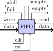
The FIFO has data and command signals for both reading and writing tokens. The FIFO is a purely synchronous system[31] i.e. all read and write operations are executed at the rising edge of the clock signal. There are also 4 status-signals available which are used to generate the feedback-signals to the nodes. Figure 3.4 shows a FIFO with all the signals.

FIFO write

data

read data empty aempty full

afull

clk rst

Figure 3.4: FIFO implementation

The write and read signals are synchronous command-signals for reading and writing tokens. These commands are only executed at the rising edge of the clock. The full and empty signals are asserted when the FIFO is full or empty. The signal afull is asserted by the FIFO when there is only one place available(almost-full). A similar signal is asserted when the FIFO is almost empty (aempty). Theempty signals are used in the firing rule to check the availability of tokens on the input i.e. a node may not execute if any of the required arcs is empty. Note that full and empty cannot be omitted because the FIFO may become completely full or empty. This is caused by backpressure when a dataflow node does not read until an arc is completely filled, or does not write until an arc is completely empty. Without the full

and empty signals of the FIFO, the next state cannot be predicted correctly and the Data Flow Graph deadlocks.

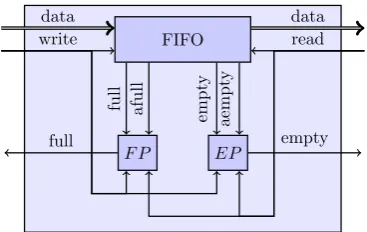
Arcs from dataflow graphs are implemented using the mentioned FIFO combined with two additional modules called next state predictors. These state predictors predict, based on the status signals of the FIFO and the read and write signals, what the next state of the node should be. The full and the empty signals are predicted by the Full Predictor (FP) and Empty Predictor (EP) respectively. All status signals from the FIFO, the full and

(20)

CHAPTER 3. DATAFLOW GRAPHS IN VHDL 14

bits for the data signals depends on what type of data should be stored on the arcs. Figure 3.5 shows the implementation of the arc.

FIFO

F P EP

full _afull

empt

y

aempt

y

data data

full empty

[image:20.595.205.389.163.279.2]

write read

Figure 3.5: Arc with next-state prediction

The arc depicted in figure 3.5 shows the two predictorsF P andEP. These are pure combinatorial blocks which means that the full and empty signals are valid before the next rising edge of the clock. These signals are then used by the state machines of the nodes to implement the firing rule. The expression of equation (3.1) predicts when the FIFO is full and equation (3.2) predicts when it is empty.

f ull= (_¬read_∧f ull)_∨(_¬read_∧write_∧af ull) (3.1)

empty= (_¬write_∧empty)_∨(_¬write_∧read_∧aempty) (3.2)

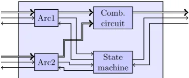
Every node in the dataflow graph implemented in VHDL, is composed of an arc on every input, a combinatorial block which performs the operation and a state machine which implements the firing rule with backpressure. Fig-ure 3.6 shows the components in a complete dataflow node. All the inputs are constructed using arcs such that tokens can be stored. Note that tokens are now stored inside of the dataflow node instead of on the edge in between two dataflow nodes. On arcs, backpressure guarantees that tokens cannot be lost and is implemented using the full signals. The firing rule with backpressure is implemented using a simple state machine shown in figure 3.2. This state machine uses the empty signals from all the input arcs and the full signals from the destination node as control signals.

(21)

CHAPTER 3. DATAFLOW GRAPHS IN VHDL 15

Arc1

Arc2

Comb. circuit

[image:21.595.200.393.125.205.2]

State machine

Figure 3.6: Components in dataflow node with backpressure

3.3

FIFO-size for full throughput

Consider the implementation of a simple dataflow graph containing two nodes shown in figure 3.7. The size of the FIFO contained within the arc can be one element. Both producer and consumer change their state based only on the state of the arc. During startup of the system, the arc is empty and both state machines (SM1 and SM2) are in the waiting state. The producer

makes a transition to the processing state because the arc is empty. The consumer remains in the waiting state because the arc contains no tokens yet. After a rising edge of the clock, the predictors in the arc predict that the producer should go to the waiting state and the consumer should go to the processing state. After yet an other rising edge, the predictors produce the reverse prediction, now the consumer should wait while the producer should go to the processing state. The effective performance of a node containing a combinatorial function is therefore one token per two clock cycles. This is because there is only one position available and both nodes can not read and write at the same time. Although it is possible to achieve full performance with only a single position in the arc, it requires a combinatorial path through all nodes. An example is a pipeline, the whole pipeline should stall if there is no storage available anymore.

Producer Consumer

SM1 arc SM2

data write

full

data empty read

Figure 3.7: Dataflow graph for full performance

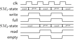
Figure 3.8 shows the timing behavior of the dataflow graph shown in fig-ure 3.7. Before the first rising edge of the clock, both state machines are in the waiting state. During the rising edge, the state machine of the producer (SM1) goes to the processing state (proc) because the arc is not full. The

state machine of the consumer (SM2) remains in the waiting (wait) state as

(22)

CHAPTER 3. DATAFLOW GRAPHS IN VHDL 16

clk

SM1-state wait proc wait proc wait

write full

SM2-state wait proc wait proc

[image:22.595.217.375.123.208.2]

read empty

Figure 3.8: Toggling behavior when size of FIFO is 1.

in the arc informs the producer to go to the wait state again because the arc will be full in the next state. After the second rising edge of the clock, the consumer is in state proc. The empty prediction in the arc makes sure that, during the third rising edge of the clock, SM2 goes to statewait again.

Because the FIFO can contain at most one token, both the producer and consumer have to wait before the arc is available for them. This results in the toggling behavior as shown in figure 3.8. The arc is the bottleneck because it will be full after a single write. The maximum throughput is therefore restricted to one token per two clock cycles.

By increasing the size of the FIFO to two, the toggling disappears. The full-signal generated by the full-predictor now remains false because the con-sumer starts reading during the writing of the second token. Writing a token to the arc and reading a token at the same time has no effect on the number of tokens stored in the arc. The producer and consumer can therefore continue at full speed of one token per clockcycle. Figure 3.9 shows that after one clock cycle both the full and empty signal remain low. Both SM1 and SM2 can

therefore remain in the procstate which results in full performance.

clk

SM1-state wait proc

write full

elements in arc 0 1

SM2-state wait proc

read empty

Figure 3.9: Full throughput when size of FIFO is 2.

[image:22.595.210.379.492.587.2]

(23)

4

Analysis of algorithms

A shown in the chapter with the background information, the beamformer used in LOFAR consists of three major algorithms, Fast Fourier Transformation (FFT)s, complex multiplications and Finite Impulse Response (FIR)-filters. In chapter 6, these algorithms are used to analyse the performance of both implementations of the FlexCore. First, this chapter explores the regulari-ties that can be found in these algorithms. The goal is to exploit locality of reference by reducing the communication overhead caused by the matching procedure as explained in the chapter on background information (chapter 2). The overlap among the three algorithms is used to design an Arithmetic Logic Unit (ALU) which is able to perform the three algorithms. The three algo-rithms are analysed and than combined into a single dataflow graph which will form the major part of the ALU.

4.1

Complex multiplication

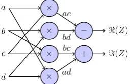
Complex multiplications are used in both the FFT and phase shifts. Consider a complex multiplication Z =Z1×Z2 where Z1=a+iband Z2=c+id are

both complex numbers. By writing down the multiplication in the canonical form(equation (4.1)), the number of real valued operations can be found.

Z =Z1×Z2 ⇒(a+ib)×(c+id) =ac+iad+ibc−bd=ac−bd+i(ad+bc) (4.1)

a b c d

×

−

+

<(Z)

=(Z)

[image:23.595.233.361.597.680.2]

ac bd bc ad

Figure 4.1: DFG of complex multiplication

(24)

CHAPTER 4. ANALYSIS OF ALGORITHMS 18

Both the real part<(Z) =ac−bdand the imaginary part=(Z) =ad+bc

require two real valued multiplications which makes a total of four multiplica-tions, one addition and one subtraction. The corresponding DFG is depicted in figure 4.1.

4.2

FFT

As shown in the background information of chapter 2 and in [24], the Fast Fourier Transformation (FFT) is the algorithm which splits the spectrum in small parts such that phase shifts can be easily implemented. An FFT is a computationally efficient implementation (N log2(N) operations for N input

samples instead of N2) of the Discrete Fourier Transform (DFT). In this section, the FFT is derived from the definition of the DFT. From the FFT the basic building block, called a butterfly operation[21], is derived which is the smallest FFT possible. The butterfly operation will be combined with a partial FIR filter and the complex multiplication in section 4.4 to form an ALU which can execute them all.

First consider the definition of the DFT shown in equation (4.2). This function operates on blocks ofN samples from which a spectrum ofN points is calculated.

ˆ

Xk= N−1

X

n=0

xne−

2πi N nk=

N−1

X

n=0

xnW

kn

N, wherek= 0, . . . , N−1 (4.2)

Where the complex factorWknN is called a twiddle factor[21]. The sum of

equation (4.2) can be split in an odd and even part:

ˆ

Xk= N/2−1

X

m=0

x2mW

k2m

N +

N/2−1

X

m=0

x2m+1W

k(2m+1)

N (4.3)

By looking only at the first part of the spectrum and using the identity

Wk2Nm = W km

N/2_{, the definition of the FFT can be found as shown in}

equa-tion (4.4).

ˆ

Xk = N/2−1

X

m=0

x2mW

km

N/2 ₊_WNk

N/2−1

X

m=0

x2m+1W

mk

N/2_, _k_{= 0}_{, . . . ,}N

2 −1 (4.4)

The second half of the spectrum is given by equation (4.7) using the fol-lowing equalities:

W

m(k+N/2)

N/2 ₌_W

mN/2 N/2 _W

mk N/2 ₌_W

mk

N/2 _(4.5)

Wk+NN/2 =W N/2

N W

k

N =−W

k

(25)

CHAPTER 4. ANALYSIS OF ALGORITHMS 19

ˆ

Xk+N/2 =

N/2−1

X

m=0

x2mW

km N/2−_WNk

N/2−1

X

m=0

x2m+1W

mk

N/2_, _k_{= 0}_{, . . . ,}N

2 −1 (4.7)

By using N = 2 in equation (4.4) and equation (4.7), the smallest FFT possible, the butterfly operation, can be found. This gives two complex results

ˆ

X0 and ˆX1.

ˆ

X0 = 2/2−1

X

m=0

x2mW

km

2/2 ₊_WNk

2/2−1

X

m=0

x2m+1W

mk 2/2 ₌_x

0+W

k

Nx₁ (4.8a)

ˆ

X1 = 2/2−1

X

m=0

x2mW

km

2/2 ₋_WNk

2/2−1

X

m=0

x2m+1W

mk 2/2 ₌_x

0−W

k

Nx₁ (4.8b)

This formula can be directly translated into a dataflow graph as shown in figure 4.2a which gives the butterfly structure. Because the twiddle factor can be implemented using a complex multiplication, the graph of figure 4.1 is reused. Figure 4.2b shows the butterfly structure for real valued signals using the graph for complex multiplications. The total number of operations re-quired to execute a butterfly operation is four multiplications, three additions and three subtractions.

x0

x1 _WNk −

+

ˆ X1

ˆ X0

(a) Butterfly of complex signals

<(x0)

=(x0)

<(x1)

=(x1)

<(W)

=(W)

× × × × − + − − + +

=( ˆX1)

<( ˆX1)

=Xˆ0)

<( ˆX0)

Compl. multiplication

(b) Butterfly of real valued signals

Figure 4.2: Complex and real valued dataflow graph og the butterfly operation

4.3

FIR filter

(26)

CHAPTER 4. ANALYSIS OF ALGORITHMS 20

is constructed[22],[24]. A FIR filter is a linear combination of the current and previous samples as shown in the following recurrence equation:

yn= N−1

X

i=0

Ci×xn−i (4.9)

N is the number of filter taps andN−1 is the order of the filter. Analysis of FIR filters is usually done in theZ domain where a FIR filter is expressed as a polynomial. Equation (4.10) shows the polynomial of a FIR filter.

H(z) =CN−1∗ZN−1+CN−1∗ZN−1+...+C1∗Z−1+C0 (4.10)

This function is called the transfer function of a filter and it shows the sum from equation (4.9) implemented in the Z domain. Every term Cn ∗

Z−n represents a coefficient being multiplied with a delayed input sample. Multiplying a signal with Z−n _{corresponds to delaying the input signal with}

nsamples. Equation (4.10) can be translated into a dataflow graph as shown in figure 4.3 which is called the standard form [21].

×

C0

z−1

×

+ C1 In

z−1

×

+ CN−2

z−1

×

+ CN−1

Out

Figure 4.3: FIR Filter

Any valid mathematical rearrangement of the transfer function of equa-tion (4.10) gives the same filter response but results in another structure of the dataflow graph. The rearrangement shown in equation (4.11) of the transfer function results in the dataflow graph of figure 4.4 which is called the trans-posed form[21].

H(z) =C0+Z−1(C1+Z−1(C2+...+Z−1(CN−2+Z−1CN−1)...)) (4.11)

(27)

CHAPTER 4. ANALYSIS OF ALGORITHMS 21

×

CN−1

z−1 +

×

CN−2 In

z−1 +

×

C1

z−1 +

×

C0

Out

Filter-tap

Figure 4.4: FIR Filter in transposed form

Partitioning and sequential execution

By partitioning the filter into smaller slices, they can be executed sequentially. This process is called folding [32]. The size of each slice is chosen to be 4 taps such that the number of multiplications is the same as for complex multiplications. Every tap consists of a multiplier and adder i.e. a single slice consist of 4 multipliers and 4 adders. The number of multiplications is therefore the same for filtering, complex multiplication and the butterfly. An example of a sliced FIR filter is shown in figure 4.5.

12 taps FIR In

Out

(a) 12 taps FIR

P 4 FIR 4 FIR 4 FIR C

a0 a1 a2 _a

5 a4

a3

(b) Sliced FIR

Figure 4.5: Slicing of FIR filter

The 12-tap FIR filter shown in figure 4.5a is partitioned in_d12₄ _e= 3 slices as shown in figure 4.5a. These slices are executed sequentially by an ALU which is able to execute a single slice at once. The results of a slice are forwarded to the next slice or the output. The input data for a slice comes either from another slice or from the input of the filter.

Figure 4.6 shows the flow of tokens in the sequentialized filter. Every arc in the dataflow graph of figure 4.5b is translated into a bufferanof figure 4.6. In order to support two incoming and two outgoing streams of data for the four taps FIR, the arcs are divided into two groups (a0−2 and a3−5) that

can be used in parallel. A single multiplexer is used to select between the producer P and the FIR which are the only producers for a0−2. The data

from group a3−5 is forwarded to the lower input of the FIR or the consumer

C. The upper input of the FIR accepts only data from a0−2 and the lower

output only produces data for a3−5, this all follows from the dataflow graph

of figure 4.5b.

(28)

CHAPTER 4. ANALYSIS OF ALGORITHMS 22 4 FIR P C a0 a1 a2 a3 a4 a5 m0 m1 m2 m3 m4 m5

(a) Phase 1

4 FIR P C a0 a1 a2 a3 a4 a5 m0 m1 m2 m3 m4 m5

(b) Phase 2

(c) Phase 3

(d) Phase 4

(e) Phase 5

Figure 4.6: Sequential execution of FIR filter.

phases1_{, one phase for every node. During phase 1, only the producer} _P

is active and sends data to arc a0 via multiplexersm0 and m2. Note that P

may send any number of tokens to the arc as long as it fits in the arc and when all other nodes in the graph consume and produce the same number of tokens. In phase 2 (figure 4.6b), the tokens sent into a0 are used by the first

filter slice.

During phase 2 the first filter slice is active which consumes all tokens in arca0 (selected by multiplexer m3) and produces tokens in arca1 and a3. As

can be seen in figure 4.6b,a1 and a3 are selected by multiplexersm2 and m4.

m0 now selects the upper output of the FIR slice instead of the producerP.

Note that the lower input of the slice is not shown here but it can be fed with a stream of zeros.

During phase 3 a FIR slice is executed which requires two input arcs and two output arcs. Again, the input arcs are selected by m3 and m5 and the

output tokens are forwarded by m2 and m4. Corresponding to the DFG of

figure 4.5b, tokens are consumed from a1 anda3 and and the resulting tokens

are sent to arca2 anda4such that the last FIR slice can consume these again.

The tokens produced in phase 3 are consumed by the last filter slice in phase 4 (figure 4.6b). Multiplexers m3 and m5 are now selecting a2 and a4

which contain the tokens produced in the previous phase. These tokens are now consumed by the slice which produces output tokens which are sent to a single arc,a5. During the last phase, figure 4.6e, multiplexers m1 and m5 are

configured such that tokens froma5 can be consumed by the consumerC.

Every time a new slice is scheduled the corresponding set of 4 coefficients has to be supplied too. Although the flow of tokens can be implemented like shown in figure 4.6, the filter-state is not preserved. Every slice contains

1_{Note that phase 1 and 5 can be combined in a single phase as no multiplexers and arcs}

(29)

CHAPTER 4. ANALYSIS OF ALGORITHMS 23

four delay elements (z−1) which contain intermediate results from previous slice executions. This means that every slice has a corresponding state which has to be loaded before it may consume tokens and execute. The ALU that executes the FIR operation therefore must be able to load the complete state of the slice first. By adding a multiplexer in front of every register (z−1), the state can be loaded using the StateIn inputs as depicted in figure 4.7. The state comes from a module outside of the ALU which will be introduced in section 5.3.

z−1 +

×

Cn+0

StateInn+0

StateOutn+0

z−1 +

×

Cn+1

StateInn+1 StateOutn+1

z−1 +

×

Cn+2

z−1 +

×

Cn+3

Outt

Outb

Inb

Int

Figure 4.7: FIR slice with state loading

As shown in figure 4.7 the state of a FIR slice is loaded using theStateInn inputs. During loading of the state, the input of the registers is connected to the StateInn input. During normal execution the multiplexers are in the upward position such that the slice of figure 4.7 resembles the transposed FIR structure of figure 4.4. When the next slice should be executed, the changed state of the current slice has to be stored. For this, the StateOutn outputs are used. Again, the state of the slices is stored outside of the ALU.

4.4

Merge of algorithms

(30)

CHAPTER 4. ANALYSIS OF ALGORITHMS 24

+/- + + +

× × × ×

z−1 _z−1 _z−1 _z−1

− −

In3

In2

In1

In0

StateIn0

StateIn1

StateIn2

StateIn3

C0 C1 C2 C3

Out0 Out1 Out2Out3

Figure 4.8: Merged DFGs for ALU design

Figure 4.9 shows the graph configured as a FIR slice. Note again that executing a filter slice requires two phases, first the slice-state is loaded using the Staten signals while execution happens during the second phase. The state can be loaded by setting every multiplexer in front of a register (z−1_),

in the down position. During normal execution the multiplexers are in the upward position as shown in figure 4.9. The inputs Int,b, coefficients C0,1,2,3

and outputs Outt,b match with the slice shown in figure 4.7.

+/- + + +

× × × ×

z−1 _z−1 _z−1 _z−1

− −

Inb Int

Staten+0

StateInn+1

StateInn+2

StateInn+3

C0 C1 C2 C3

Outt Outb

Figure 4.9: Configuration for FIR slice

By selecting the multiplexers as depicted in figure 4.10, the graph is con-figured as a complex multiplier. Z1 is presented on the inputs while Z2 is

presented as constants for the multipliers. Note that both the real and imag-inary part of Z2 are duplicated as input constants. A complex multiplication

(31)

CHAPTER 4. ANALYSIS OF ALGORITHMS 25

not used. The result Z is presented on the output using two multiplexers. The remaining outputs from the subtractors are only used in the butterfly operation.

− + + +

× × × ×

z−1 _z−1 _z−1 _z−1

− −

=(Z1)

<(Z1)

<(Z2) =(Z2) <(Z2) =(Z2)

<(Z) =(Z)

Figure 4.10: Configuration for complex multiplication Z =Z1×Z2

Figure 4.10 shows the configuration when the butterfly operation is se-lected. The twiddle factor of the butterfly operation is implemented using a complex multiplication so the constants are duplicated again over the mul-tipliers. Also the butterfly operation is state-less so the registers with the corresponding multiplexers are not used. This selected mode shows the exe-cution of the graph of figure 4.2b.

− + + +

× × × ×

z−1 _z−1 _z−1 _z−1

− −

=(x1)

<(x1)

<(x0)

=(x0)

<(W) =(W) <(W) =(W)

<( ˆX0) =( ˆX0) <( ˆX1) =( ˆX1)

(32)

5

FlexCore architecture

This chapter presents the design of the FlexCore. The FlexCore has been designed in two phases: first a standard dataflow architecture including back-pressure has been designed to act as reference design. This is presented in section 5.1 and section 5.2. During the second phase elaborated in section 5.3, the architecture is extended such that the merged dataflow graph presented in chapter 4 can be used as ALU for efficient execution of beamforming oper-ations.

5.1

Overview of architecture

Figure 5.1 shows an overview of the FlexCore with its modules. The FlexCore has a similar circular structure as the early dataflow architectures presented in [12],[17] and [19]. It consists of three main modules, the Router which routes internal tokens of the FlexCore and tokens from the NoC, the Dispatcher which implements the firing of nodes based on the availability of tokens and the ALU which performs the actual calculations.

The router manages the flow of tokens from the NoC and for the processor itself. Every token that should be processed by the Router has a value and a destination-address. Based on this address the router can determine whether to send an incoming token to the dispatcher or to the NoC. Tokens flowing trough the processor have the following format:

token={globalAddress, localAddress, inputAddress

| {z }

destination

, value} (5.1)

As shown in the expression above, the address consists of three parts. The

globalAddress is used by the router to determine whether a token should be sent to the dispatcher or to the NoC. A global address is assigned to the FlexCore, this means that the router forwards an incoming token to the dispatcher whenglobalAddressof that token is equal to the address assigned to the FlexCore. When this is not the case the router sends it to the NoC. The localAddress field is used to address nodes of the DFG according to the

(33)

CHAPTER 5. FLEXCORE ARCHITECTURE 27

ETS principle explained in figure 2.3. inputAddressindicates to which input of the node in the DFG, the token should be sent. Thevaluefield of the token contains the actual data. All data values in the FlexCore are 16 bit signed numbers which is a common wordlength for DSP applications[33],[34]. The general architecture of the FlexCore is shown in figure 5.1.

Dispatcher

NoC Router

Presencebit Memory

Program Memory

Token Store

ALU progr.

interface

dest. dest. value

FlexCore

Figure 5.1: FlexCore architecture overview

The dispatcher is responsible for matching tokens and sending them with an instruction to the ALU. The router sends tokens to the dispatcher which implements the ETS principle. The dispatcher itself is constructed using three sub modules: the presence bit memory, program memory and token store.

The presence bit memory uses only the local address from the incoming token. Based on this local address a presence bit is fetched from the memory. This bit is sent to both the program memory and the token store. During every access of a presence bit, the value is inverted. When the presence bit being sent out containstrue, a match is found and an instruction is dispatched on the ALU.

The program memory accepts both the local address from the incoming token as well as the presence bit produced by the presence bit memory. When the presence bit contains the valuetrue, the instruction addressed by the local address should be scheduled. This instruction is stored in a memory where ev-ery location contains the instruction and several destination addresses. These destination addresses are the nodes to which the result of the operation should be sent as explained in figure 2.3. When the presence bit is false, the instruc-tion should not be scheduled. Therefore both the address and the presence bit are removed from the arc and no tokens are produced by the program memory.

(34)

CHAPTER 5. FLEXCORE ARCHITECTURE 28

value true. The token store accepts three inputs, a presence bit, the value of the incoming token and the local destination address of that token. When the presence bit is false no match has occurred so the incoming token is stored in the memory of the token store addressed by the local destination address from the incoming token. When both operands are available i.e. a match occurs, a presence bit containing true is received by the token store. The token store sends both the incoming token and the previously stored token to the ALU. When two tokens are sent to the same input of a node, the dispatcher interprets this as a match which is not the case. The input data should be restricted such that this situation will never occur.

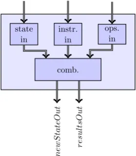
The ALU performs all the calculations and accepts the instruction and destination(s) from the program memory. The operands are received from the token store. When the operands and the instruction are available in the FIFOs, the firing rule is satisfied and the ALU starts the execution. The resulting value is sent sequentially to all destinations (max. 4), the operations may take 4 clockcycles to complete from which only one cycle is needed for the calculation.

5.2

Implementation

ALU

The first design of the FlexCore contains a small ALU which is only able to perform additions, subtractions and multiplications. The ALU has two inputs, one for receiving instructions and one for the operands. As with every input of a dataflow node, backpressure and buffering is supported by using arcs. The firing rule and execution of this module is implemented by a statemachine. The execution may only start when there is an instruction on the instruction arcinstr. arc, when a set of operands1is available in the operands arcops. arc

and if there is still space available on the arc to which the result will be sent (Router). The firing condition then becomes:

f ire=¬empty(instr. arc)∧ ¬empty(ops. arc)∧ ¬f ull(Router) (5.2)

The general structure of the ALU and the firing rule implemented by the state machine shown in figure 5.2.

The ALU can execute nodes from a dataflow graph with up to four des-tinations. The result, produced by the operation, is therefore sent to all the nodes in the dataflow graph to which an output of the producing node is connected. The output of the ALU however only allows one token per clock cycle to be sent to the router. The tokens are therefore sent sequentially to all destinations.

(35)

CHAPTER 5. FLEXCORE ARCHITECTURE 29

wait

proc f ire

¬f ire/updateP tr()

¬f ire

f ire/updateP tr()

(a) Statemachine

instr. arc

ops. arc

state ma-chine

comb. func-tion

(b) Internal structure

Figure 5.2: Implementation of ALU

The number of destinations destCnt is encoded in the instruction which has the following format: (instr, destCnt, dest0, dest1, dest2, dest3) whereinstr

can bemult,addorsubanddestCntmust be in_{1,2,3,4_}. The statemachine iterates overdestCntdestinations to which the result will be sent. Every time the statemachine leaves theproc state, a pointer pointing to the current desti-nation is updated. Updating the pointer is performed byupdateP tr() shown in algorithm 1.

Algorithm 1: Implementation of updateP tr() if curDest=destCnt then

1

curDest_←dest0

2

else

3

curDest←curDest+ 1

4

After a reset of the FlexCore,curDestis initialized todest0, i.e. during the

first cycle the first destination is always selected. After the first cycle a tran-sition is made in the statemachine whereupdateP tr() is executed. Depending on the number of destinations, destCnt, the next destination is selected or the first(dest0) for the next execution of the ALU. When the result is sent to

the last destination, both input arcs will be read such that storage is freed for the next instruction and operands.

Dispatcher

(36)

CHAPTER 5. FLEXCORE ARCHITECTURE 30

which is used by all three modules inside of the dispatcher. The f ull signal from dispatcher to router must therefore be dependent on full signals from all modules in the dispatcher. The input of the dispatcher is full when any of the f ull signals of the internal modules are set. The following approach is applied to the signal coming from the presence bit memory: the f ull signal going into the presence bit memory should be set when either the f ull signal from program memory or token store is set. The outputs of the dispatcher are simply forwarded signals from the program memory and token store. This requires no additional logic.

Presence bit memory

Detecting a match is performed by the presence bit memory. For binary (only two inputs per node) dataflow graphs only a single bit is needed per node in the DFG[19]. Initially, all presence bits in the memory are reset when the whole FlexCore is reset. This means that for all nodes in the DFG, no token has yet been received. When a token arrives at one of the inputs, the bit is set. Based on the presence bit and a new incoming token addressed to the same node, a match is found and the presence bits memory will inform the program memory and token store.

wait

proc f ire

¬f ire/invertBit(dest)

¬f ire

f ire/invertBit(dest)

(a) Statemachine

dest. arc

state ma-chine

RAM

Figure 5.3: State machine and internal structure of the presence bit memory

The presence bit memory has only a single input, the destination address of the token sent from router to dispatcher is used. This address is, conform to the dataflow model, stored in an arc (see structure of the module in fig-ure 5.3b). The firing rule and reading from the arcs is implemented by the statemachine shown in figure 5.3a. The firing rule states:

(37)

CHAPTER 5. FLEXCORE ARCHITECTURE 31

For every incoming destination address, the bit pointed by that address is inverted. Although only a single bit for every node in the DFG is required, the number of tokens that can be stored on an arc of the DFG is restricted to one. A match is found when an address of the presence bit memory is addressed twice. The input to which the token should be sent is ignored to save hardware. The inputs to which the tokens forming a match should be sent, is determined in the token store.

Program memory

The program memory selects an instruction when a match is found in the presence bit memory. Which node should be executed is determined by the destination address from the token sent from router to dispatcher. When the presence bit memory reports that no match is found, the program memory simply does not send an instruction to the ALU. Additional to the dataflow in- and outputs, the program memory has an external programming interface. This is used by the testbench to load the dataflow graph (the program that should be executed) into the FlexCore. The internal structure of the program memory can be seen in figure 5.4b.

wait

proc f ire

¬f ire

f ire

(a) Statemachine

dest. arc

presbit arc

state ma-chine

RAM

instr addr write

Figure 5.4: State machine and internal structure of the program memory

The state machine shown in figure 5.4a is only used to implement the firing rule. The actual selecting of the memory is performed combinatorially during theproc state. When the presence bit memory sends a token containing true

i.e. a match is found, the instruction addressed by the incoming destination address is sent to the ALU. Whenfalse is received, the address is ignored and nothing is sent to the ALU. An instruction in the program memory has the following format: (instr, destCnt, dest0, dest1, dest2, dest3), which is exactly

(38)

CHAPTER 5. FLEXCORE ARCHITECTURE 32

f ire=_¬empty(dest. arc)_{∧ ¬}empty(presbit arc)_{∧ ¬}f ull(ALU) (5.4)

Token store

The token store is responsible for storing tokens on the arcs of a DFG until all tokens for a node are available. The nodes of the DFG always have two inputs, the token store therefore only has to be able to store one token per node. When the second token of a node arrives, a match is found and the incoming token combined with the token with the same address (destination in the DFG) form the set of operands. Tokens triggering a match therefore never have to be stored but are directly forwarded to the ALU. The token store always stores the first arriving token for a node, independent to which input the token is sent. Only the value contained within the token is stored in the token store because the input can be determined when the second token arrives. Because of this, the standard FlexCore only supports two input nodes in the DFG, the input to which the first token should be sent is the inverse of the input to which the second is sent: If the first token is sent to the left input of the destined node, the second token is sent to the right input and vice versa. This imposes a restriction on the arrival of tokens: only one token can be stored on an arc. This is caused by the fact that the token store can only store one token per node and the presence bit memory reports a match when two tokens with the same address arrive (independent of whether the are sent to the same input). The order in which two operands for a node arrive is not restricted, a functionorder() makes sure the the operands are sent to the correct input.

The statemachine for the token store is like all others: processing starts only when the firing rule is satisfied. The token store requires three incoming tokens: a presence bit, the destination of the incoming token and the value. The firing rule then becomes:

f ire=_¬empty(presbit arc) _{∧ ¬}empty(dest. arc)_∧

(39)

CHAPTER 5. FLEXCORE ARCHITECTURE 33

wait

proc f ire

¬f ire

f ire

(a) Statemachine

presbit arc

dest. arc

val. arc

state ma-chine

RAM

order

Figure 5.5: State machine and internal structure of the token store

Algorithm 2: Algorithm for the token store while truedo

1

while_¬f ire do

2

wait;

3

if presbit=truethen

4

write_←true;

5

operandsOut_←order(dest, value, loadF romRAM(dest));

6

else

7

write←f alse;

8

operandsOut_{← ∅};

9

storeInRAM(value, dest);

10

Router

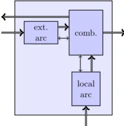
The router is the only module in the FlexCore without a statemachine. This is because the firing rule depends on the destination to which an incoming token should be sent. If for example a token should be sent to the dispatcher, the firing rules require that there is space at the input of the dispatcher. When a token should be sent out of the processor, firing does not depend on the dispatcher but on the router output. In order to avoid a complex statemachine, the routing is performed combinatorially.

(40)

CHAPTER 5. FLEXCORE ARCHITECTURE 34

the core. Tokens from outside the core can only enter if there is space in the input of the router. Because the local input of the router has priority over the external input, external tokens are accepted only if temporarily no tokens are in the local input. This means that the dispatcher is able to accept data from outside of the core again. Figure 5.6 shows the structure of the router.

comb. ext.

arc

[image:40.595.237.362.205.332.2]

local arc

Figure 5.6: Combinatorial implementation of firing rule in router

For the availability of tokens in the arcs, three basic cases can be distin-guished: there is data available in the local arc, there is data in the external arc or there is no data at all. The algorithm of the router in shown in algorithm 3.

Algorithm 3: Algorithm for routing tokens if _¬empty(localArc) then

1

if localT oken.dest=local_{∧ ¬}f ull(Dispatcher)then

2

dataT oDispathcer←localT oken;

3

else if localT oken.dest=external_{∧ ¬}f ull(External) then

4

dataRouterOut←localT oken;

5

else if _¬empty(extArc)_{∧ ¬}f ull(Dispatcher)then

6

dataT oDispathcer←extT oken;

7

else

8

wait for data;

9

5.3

Extended architecture for beamforming ALU

(41)

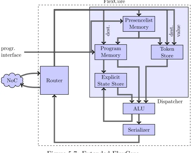
CHAPTER 5. FLEXCORE ARCHITECTURE 35

FIR slice and a complex multiplication require two inputs while the butterfly operation requires four inputs. Note that the complex multiplication requires two inputs because the second complex operand is supplied as a constant from the program memory. Secondly a FIR slice has state which has to be supplied to the ALU every time a slice is executed. After execution the FIR slice has a new state and it should be stored for subsequent execution of the same slice. First the required changes to the dispatcher are elaborated in order to support the matching for different numbers of inputs. This is followed by the handling of state from FIR slices. After that the implementation of the modules is explained. The extended architecture is shown in figure 5.7.

Dispatcher

NoC Router

Presencelist Memory

Program Memory

Explicit State Store

Token Store

ALU

Serializer progr.

interface

[image:41.595.147.456.277.523.2]

dest. dest. value FlexCore

Figure 5.7: Extended FlexCore

Overview

The general structure of the extended FlexCore is very similar to the architec-ture shown in figure 5.1, except the naming and additional modules. Tokens from outside of the FlexCore are sent to the router which forwards these to the dispatcher. The matching process takes place in the dispatcher by checking whether all operands are available. When this is the case, the Presencelist memory reports a match which is sent to both theProgram memory and the

(42)

CHAPTER 5. FLEXCORE ARCHITECTURE 36

the instruction is scheduled. The operands for the instructions are stored in the Token Store until a match is found. All operands, the instruction and an optional state are then sent to the ALU which performs the instruction. Several tokens at once are produced by the ALU which are sent sequentially to the router by theSerializer. The router of the standard FlexCore is therefore reused.

Changes to Dispatcher

Because the number of inputs for nodes of a DFG for the extended FlexCore may differ, the matching cannot be based on a single presence bit anymore. When a node has four inputs, four operands must be available while a two input node only requires two operands. The presencelist memory therefore must know if the addressed node has four or two inputs. This is solved by adding an additional field (type) to the elements of the presencelist memory. This type field represents how many inputs that particular node has and is set during programming of the FlexCore. Every element now consist of a type field and a list of bits where every bit represents the availability of an operand. The extended FlexCore uses the same addressing scheme from ETS as the standard FlexCore.

The Explicit State Store (ESS) is added to the dispatcher to hold the state information for certain nodes in the DFG. When the program memory encounters a FIR slice, the state address for that instruction is sent to the ESS. The ESS then selects the state for the slice and sends it to the ALU. After execution, the state of the slice is changed and the ALU sends it back to the ESS for the next execution of the same node.

Another difference with the standard FlexCore is that instructions now also contain coefficients for the FIR slices, and complex numbers for complex multiplications and twiddle factors. This is done to restrict the number of inputs for nodes in the DFG and therefore simplifying the matching (a maxi-mum of four tokens now have to be matched instead of six). All elements in the program memory now have a set of four coefficients.

Implementations

Presencelist memory

Instead of single bits, the presencelist memory contains a list of bits for match-ing (one bit for every input). Based on a type field the presencelist memory can determine whether all operands are available. A single element has the following structure: (type,(bit0, bit1, bit2, bit3)) where type can be twoInputs

(43)

CHAPTER 5. FLEXCORE ARCHITECTURE 37

occurs when all bits, except the one destined by the incoming token, are set. The presencelist memory sends a token containingtrue to the program mem-ory and token store when a match is found or false otherwise. The interface of the presencelist memory to other modules is not changed. The algorithm of the presencelist memory is shown in algorithm 4.

Algorithm 4: Algorithm for the presencelist memory while truedo

1

while¬f ire do

2

A dataflow architecture for beamforming operations