The storage and retrieval of sensor data and its annotations

UNIVERSITY OF TWENTE

MASTER THESIS

The Storage and Retrieval of Sensor Data and its Annotations

Bart Sikkens

Department of Computer Science

Groningen, May 31, 2010

The focus of this thesis is on the storage part of a sensor management system. Sensor data can already be enormous, but because every measurement stored can also contain multiple

annotations the total size can really explode. Besides this, annotations are not necessarily bound to a single measurement, but can also be attached to multiple sensors and on time spans. This creates challenges in storing the data efficiently while also maintaining efficient retrieval. On the retrieval side there are all kinds of queries possible on the sensor data, annotations, time or combinations of those. To provide efficient storage for all these types of queries makes things even more challenging, because every storage method has its advantages and disadvantages.

1. Introduction... 6

1.1. Problem description... 6

1.2. Research goal and contribution ... 6

1.3. Research structure ... 6

1.4. Research questions ... 7

1.5. Research scope ... 7

2. Detailed problem description ... 8

2.1. Annotation and query types... 8

3. Related work ... 9

3.1. Relational storage... 9

3.2. Column databases... 12

3.3. Summary ... 13

4. Detailed approach ... 15

5. Case... 17

6. Storage of sensor data and annotations ... 18

6.1. Relational storage... 18

6.2. Column database storage... 21

6.3. Storage models to be used in scalability experiments... 22

7. Retrieval of sensor data and annotations... 23

7.1. Types of queries ... 23

7.2. Proposed query language ... 23

7.3. Translation rules... 23

8. Scalability testing of storage models ... 25

8.1. Data set for scalability testing of storage models... 25

8.2. Query set for validation... 27

8.3. Experiment design... 32

8.4. Results ... 33

8.5. Conclusions ... 38

9. Implementation ... 40

9.1. Implementation requirements... 41

9.2. Implementation details ... 42

9.3. Implementation limitations ... 43

10. Scalability testing of implementation ... 44

10.1. Data set and scalability testing design... 44

10.2. Results ... 45

11. Conclusions... 47

11.1. Future work ... 48

Acknowledgements ... 49

References ... 50

Appendix A: Data manipulation details ... 52

Appendix B: Annotation adding details ... 54

Appendix C: Queries for larger data sets using luisterbuis data ... 57

Appendix D: Implementation testing details... 60

Appendix E: Measured standard deviations for experiments... 61

Appendix F: Measured standard deviations for implementation ... 62

Figure 1: Overview of involved parts ... 15

Figure 2: Detailed action plan ... 16

Figure 3: Examples of annotations over sensor data... 17

Figure 4: Graphical view of WHB08 measurements ... 35

Figure 5: Graphical view of BDBMS measurements... 36

Figure 6: Graphical view of Hypertable measurements... 37

Figure 7: Comparison between WHB08 and BDBMS on a normal scale ... 39

Figure 8: Comparison between WHB08 and BDBMS on a logaritmic scale ... 39

Figure 9: Overview of elements within the sensordataweb [Lan09] ... 40

Figure 10: Overview of classes involved for annotation support... 42

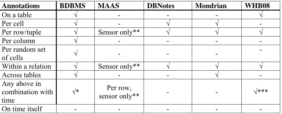
Table 1: Supported types of annotations on database level by proposed systems/methods in

literature ... 14

Table 2: Supported query types by proposed systems/methods in literature ... 14

Table 3: Example of sensor data storage per measurement type ... 18

Table 4: Example of sensor data storage per sensor ... 19

Table 5: Example of sensor data storage with all data in 1 table ... 19

Table 6: Table for weather station 1 containing annotations ... 19

Table 7: Table for storing annotation sets... 20

Table 8: Table for storing additional information about annotations... 20

Table 9: Example of sensor data and annotation storage in a 'Bigtable' system over time... 21

Table 10: Example of sensor data and annotations in a 'Bigtable' system at one specific time22 Table 11: Translation rules for SQL ... 24

Table 12: Translation rules for HQL... 24

Table 13: Schema of table containing IJkdijk data ... 25

Table 14: Overview of data set sizes... 33

Table 15: Mapping of annotation management queries to abbreviations ... 33

Table 16: Mapping of selection queries to abbreviations ... 33

Table 17: What each query does on every scale ... 34

Table 18: Execution times and peak memory usage of queries on WHB08 in seconds and bytes ... 35

Table 19: Execution times and peak memory storage of queries on BDBMS in seconds and bytes ... 36

Table 20: Execution times of queries on Hypertable in seconds ... 37

Table 21: Overview of queries and their execution plan for the sensordataweb ... 44

Table 22: Execution times of queries on implementation in seconds ... 45

Table 23: Standard deviations for WHB08 measurements ... 61

Table 24: Standard deviations for BDBMS measurements ... 61

Table 25: Standard deviations for Hypertable measurements... 61

1.

Introduction

The IJkdijk project [IJk09] is a cooperation of many companies and parties with as goals the improvement of dikes, real-time monitoring of their strength and conduct research to the use of sensor systems in early warning systems. These sensor systems consist of a multitude of sensors (video, audio, infrared, temperature, pressure etc.) which all produce sensor data at a certain frequency. Scientists involved in this project have the need to annotate this data using annotations, which say something about the measurements. While this might look like an easy task at first sight, there are complications making this a challenging task. We will start with taking a look at these complications.

1.1.

Problem description

One of the complications mentioned earlier is how to store the huge amounts of sensor and annotation data in an efficient way. Sensor data can already be enormous, but because every measurement stored can also contain multiple annotations the total size can really explode. Besides this, annotations are not necessarily bound to a single measurement, but can also be attached to multiple sensors and on time spans. This creates challenges in storing the data efficiently while also maintaining efficient retrieval. On the retrieval side there are all kinds of queries possible on the sensor data, annotations, time or combinations of those. To provide efficient storage for all these types of queries makes things even more challenging.

1.2.

Research goal and contribution

The goal of this master thesis is to take a look at the currently available methods for storing and retrieving sensor data and its annotations and test them on scalability. Due to time constraints we will have to make a selection from all available methods and we like to test at least 1 non-relational method. What we hope to contribute with this thesis is providing an overview of available methods and providing scalability numbers for a few of these methods.

Besides that we aim to create a working implementation of one of these methods. This implementation should be able to retrieve data and their annotations as well as supporting annotations in queries.

1.3.

Research structure

1.4.

Research questions

The main research question and sub questions for this research are as following:

• How can we efficiently store sensor data and its annotations in such a way that it can be queried efficiently again with different types of queries?

o What kinds of storage and storage models for sensor data and its annotations are available?

o How can we efficiently retrieve data and annotations? o Which solution has the best scalability?

1.5.

Research scope

2.

Detailed problem description

We will first take a look at what actually is the problem with storing sensor data and its annotations. The simplest approach would be to attach the annotations to the actual measurements. But measurements can have multiple annotations and a basic relational database does not support set-valued attributes. A solution is to use the first normal form (1NF) for databases, meaning we will give annotations a separate table and we create a table to connect measurements to annotations. This will result in a lot of joins when querying and redundant storage, which is inefficient. Another solution would be to use a database scheme in non-first normal form (N1NF) [JS82]. This form allows sets and therefore we can attach multiple annotations to one measurement. However relational databases do not support this form.

Next we will distinguish a number of types of annotations and queries. These will later on be used to compare all found methods in the related work section.

2.1.

Annotation and query types

We can think of different types of annotations and query types. At first we will take a look at the annotation types. We will start with annotations on different granularities of a database. Annotations can be on an entire table/relation, so every row and column in the table is annotated with a certain annotation. Whole rows/tuples and columns can be annotated, but also specific cells or a random set of cells. Annotations can be across tables, meaning that data that is split between tables is annotated using the same annotation without duplication. Annotations can also be within relations. All above mentioned types could be combined with a time element. All so far mentioned types are bound to certain sensor data. But we can also think of situations where it is hard to find to which data an annotation belongs. For example a power cut happened and all sensors went off. No data is available at that moment and

someone wants to annotate why there is no data at that time span. Because no data was created, there is no data to attach the annotation to. In this case the annotation would have to be bound to time itself.

Considering queries we can retrieve data, annotations or both. We can also add time

3.

Related work

In this chapter we will discuss related work. We will start by taking a look at relational storage and end with column databases. After discussing all literature, the summary will contain 2 tables summing up what annotations types and query types (as discussed in the previous section) are supported by which system/method.

3.1.

Relational storage

This section is divided into several categories of papers/systems. We will start looking at the similarities and differences between relational storage and XML.

XML

Where relational storage doesn’t allow the storage of a set of values in a single field, XML can store set-valued attributes. We will first have a look into literature that converts XML to a relational database. This process is called shredding.

[STH99] defines three special types of shredding using Document Type Definitions (DTDs). Normal shredding directly maps elements to relations and this creates a lot of fragmentation. The proposed solution is to use inlining, which puts as many descendants of an element as possible into a single relation. Because the traditional relational model cannot handle set-valued attributes, basic inlining uses the standard technique for storing sets in a relational database (1NF). The shared inlining method goes one step further and ensures that an element node is represented in exactly one relation. Finally the hybrid inlining method inlines even more elements. One of the conclusions this paper draws is that relational systems could more effectively handle XML query workloads with support for sets. It would reduce

fragmentation, which is a big win because most of the fragmentation they observed in real DTDs was due to sets.

The SQL/XML standard as proposed in [EM02] and [EM04] describes the mapping of SQL data to XML data. The standard has a function called XMLTable [EM04] which can

transform XML data into relational data. This function uses a form of shredding, but doesn’t require a DTD. Instead it uses XQuery [W3C01], a query language for XML, and manually chosen column names.

We can learn from this literature ([STH99] [EM02] [EM04]) that even though there are methods to convert set-valued attributes in XML to relational, the efficiency is limited by the absence of set support in the relational model. The conversion is also a lot more complicated without it. The conclusion is that the conversion of SQL to XML and vice versa has no special trick or method that could give us an advantage in storing annotations in a relational database.

BDBMS

view (automatic annotation of newly inserted data if it satisfies certain conditions) and join (attached to data across relations).

They also introduce the Mapped-Space storage scheme for efficient and compact

representation of multi-granular annotations. This scheme numbers all rows and columns and therefore annotations can be represented by rectangles. To achieve the most efficient storage, the columns with the most annotations should be next to each other, creating fewer rectangles per annotation. For this reason they created an algorithm that, based on statistics, gives the ideal mapping of columns. This process does not influence the actual physical storage order of the columns, but only the numbering of columns. Using a columns mapping quality (CMQ) metric it is decided whether it is worth re-constructing all annotations according to the new mapping. This will depend on the gain of reducing the storage overhead and I/O cost of queries compared to the cost of re-constructing.

To realise all of this, they extended PostgreSQL with new constructs and added declarative mechanisms to support adding, storing, archiving and querying snapshot, view and join annotations. The Mapped-Space schema achieves more than an order-of-magnitude reduction in storage and up to 70% reduction in the queries execution time.

For BDBMS it is important to have as much information (data and time) as possible in 1 table to make sure the number of rectangles per annotation is as low as possible. Using ‘join annotations’ it is possible to annotate across relations and hence tables, but this is a more expensive operation. For each data table multiple annotation tables can be assigned, but not the other way around. It is always possible to annotate an entire table, whole rows, whole columns or a random set of cells. If information about time can be found inside the table, it should be possible to combine all options with time. It must be said that the authors didn’t look at the time aspect, but because they extended the SQL select statement it should be possible to add time constraints in the ‘where’ clause. It is not possible to annotate on time itself. All types of queries are possible, although the time component is not discussed in the paper.

BDBMS is a very interesting and relevant system. It has the ability to store all kinds of annotations and the query language is also sufficient. The smart way of storing annotations reduces storage requirements. The only disadvantage is that the paper does not talk about support for time constraints.

MAAS

[KMP09] proposes a system for massive annotation and aggregation of sensor data. They developed a query language for efficient retrieval of data and its annotations, which can filter on both time and value ranges and supports Boolean logic operations. The language also supports adding, deleting and describing annotations. The storage is done using tables for sensor stations and tables for sensors which are linked to a station. Annotations are stored in a separate table and a relation between sensor data and an annotation is stored into another table. They use data aggregation on different levels on the time scale and annotation caching to achieve high efficiency. Their prototype features a web interface that is able to visualize data including its annotations.

In relation to our work, this system is quite relevant. It might not be able to support all types of annotations, but for sensor data it provides enough functionality. It can store multiple annotations on a measurement, but not one annotation over multiple measurements without duplication. The query language describes the functionality as we would expect from such a system.

DBNotes

[CCV05] proposes a ‘post-it note’ system for relational data. In this system it is possible to attach zero or more notes to every value in a relation. The propagation of the notes is based on provenance, which is not the focus of our research. They developed an extension to a

fragment of SQL called pSQL, which can query both data and its annotations and propagate annotations. Although the query part is relevant, the rest of the paper focuses on provenance. The original paper doesn’t describe the actual storage methods used, but [Bog05] did and also developed an alternative storage scheme for DBNotes. The original storage model created an extra attribute for every attribute in a relation in order to store the annotations. In other words, for every column an annotation column was added. This leads to redundant storage and as a direct consequence increased response time. The proposed solution is a separate relation to define the annotations present. In other words, for every table an annotation table is created storing the annotations. Besides measuring absolute performance, 2 tests were run to compare pSQL to normal SQL. The observed results were that using the default propagation, pSQL was 1 to 2 times slower than normal SQL.

[BCT04] describes work done before [CCV05] and is also about pSQL, propagation of annotations and data provenance.

DBNotes supports annotations within relations/tables. It is possible to annotate a row/tuple within a relation or one or more attributes of it. Because it is relation-based, annotations cannot be across tables. Support for time is also not available. Considering querying, data, annotations and both can be retrieved. Time support and annotation management are not supported. DBNotes main focus is on providing data provenance, which is not our focus.

Mondrian

[GKM06] proposes the Mondrian system. It has an annotation mechanism to annotate both single value and the associations between multiple values. It is able to query not only for data but also for annotations. It annotates using blocks that are put on relations. Using Boolean values it is stored which parts of the relation are affected by the annotation. The actual annotation is called a colour. The relations and annotations are stored in a new table, hence not affecting the schema of the data. Experiments done show that each colour operator costs from three to five times as much as its relational counterpart. They call the overhead not prohibitive and say it is balanced by the added value of being able to represent and query complex annotations. Planned further optimizations will further reduce the cost. Provenance was one of the motivators to develop this system, along with integrating, annotating and cross-referencing scientific databases.

DBNotes has the disadvantage of not supporting time constraints on annotations. Further it is not clear what annotation management is actually supported. It does not have the annotation flexibility of BDBMS, but it still supports some annotation types.

Other work

[WHB08] investigated ways to store both sensor and annotation data. They looked at the advantages and disadvantages. Validation was done by querying with a fixed set of queries. Their conclusion was that the sensor data storage model as later seen in Table 4, storage per sensor station, is the best solution under their assumptions (sensor are not synchronized on time, most queries contain a time constraint and more, see [WHB08]). Considering the annotation storage, they chose the storage model that will be described later in this document in the section ‘Annotation storage’ on page 19.

This research gave a nice insight into the problems arising when storing sensor and annotation data. The annotation storage model chosen is an interesting one and we will elaborate on it later on.

3.2.

Column databases

Besides XML and Relational database there is a third development in the area of storage called column databases. These databases store their data by column instead of row. This has advantages for computing aggregates and updating whole columns. We will start with taking a look at Google Bigtable, Google’s database which shares characteristics of both row-oriented and column-row-oriented databases.

Google Bigtable

Literature study shows there is only a limited amount of papers available about Bigtable and its open-source alternatives. [Goo06] describes the basics of the Google Bigtable database. This database is the method of storage behind Google projects like Google Analytics, Google Earth and Google Personalized Search [Goo08]. It is built on top of Google File System (GFS) and some other Google programs like for example Chubby Lock Service. Each table in Bigtable is “a distributed multi-dimensional sorted sparse map”, sharing characteristics of both row-oriented and column-oriented databases. The table consists of rows and columns, and each cell has a time version. There can be multiple copies of each cell with different times, so it is possible to keep track of changes over time. Columns are grouped into sets called column families. These families need to be defined before storing data, but inside them can be an unbounded number of columns, created on the fly.

Bigtable is designed to scale into the petabyte range across hundreds or thousands of machines. Also it is easy to add more machines to the system and automatically start taking advantage of those resources without any reconfiguration. One of the advantages is cheap storage of NULL values and only changes in time are stored, reducing storage overhead. [KG08] compares the performance of Hypertable and HBase, two open source alternatives for Google Bigtable. It is unknown whether the measurements done are still relevant.

Cassandra

[LM09] proposes the Cassandra system, which is the database behind the Facebook website. This system is built with continuous failure of components in mind. It does not support a full relational model, but supports dynamic control over data lay-out and form. It can handle high write throughput while not sacrificing read efficiency.

A table (also called keyspace) in Cassandra is a distributed multi dimensional map indexed by a key. The row key in a table is a string with no size restrictions, although typically 16 to 36 bytes long. Every operation under a single row key is atomic per replica no matter how many columns are being read or written into. Columns are grouped together into sets called column families, very much similar to what happens in the Bigtable [Goo06] system. Cassandra exposes two kinds of columns families, Simple and Super column families. Super column families can be visualized as a column family within a column family. Columns within a super column or simple column family can be sorted on time or name. Cassandra can store binary data and timestamps.

Facebook currently stores 50+TB of data on a 150 node cluster. [LM09-2] shows a significant performance gain over a MySQL database. On 50 GB data it took MySQL ~300ms to write and ~350ms to read, while Cassandra did it in ~0.12ms and ~15ms.

Cassandra is a robust and scalable system. It focuses on high write throughput while still reading efficiently. Sensor data on the other side is written once and never updated, but read a lot. In this sense the focus is different. The easy adding of columns makes it a very flexible system. The system is actively developed and is an interesting alternative for Bigtable.

MonetDB

MonetDB [Bon02] is a database system that is a crossover between row and column based. It shows high performance especially in data mining, OLAP and GIS applications. The

MonetDB core is usable with SQL and XQuery. For SQL there are application bindings for many programming languages and it runs on nearly any platform. MonetDB achieves its goal by innovations at all layers of a DBMS, e.g. a storage model based on vertical fragmentation, a modern CPU-tuned query execution architecture, automatic and self-tuning indexes, run-time query optimization, and a modular software architecture [CWI10].

3.3.

Summary

Annotations BDBMS MAAS DBNotes Mondrian WHB08

On a table √ - - - √

Per cell √ - √ √ -

Per row/tuple √ Sensor only** √ √ √

Per column √ - - - -

Per random set

of cells √ - - -

-

Within a relation √ Sensor only** √ √ √

Across tables √ - - √ -

Any above in combination with

time √*

Per row,

sensor only** - - √***

On time itself - - - - -

Table 1: Supported types of annotations on database level by proposed systems/methods in literature * = depending on storage model, not explicitly mentioned in paper

** = only the tables storing sensor data *** = if time is stored for each row/tuple

Table 2 shows for the proposed systems/methods in the literature what types of queries are supported. BDBMS can handle all types, but time constraints are not explicitly mentioned in the paper and neither are they tested on performance. MAAS can retrieve data and annotations, but it is not explicitly mentioned that the combination of those two is also possible. Both DBNotes and Mondrian support retrieving data, annotations and both. Mondrian also has some annotation management. Both cannot handle time constraints. WHB08 can retrieve data, annotations, both and use time constraints if the time is stored for each row.

Type of query BDBMS MAAS DBNotes Mondrian WHB08

Get data √ √ √ √ √

Get annotations √ √ √ √ √

Get both √ ?** √ √ √

Time constraints √* √ - - √****

Annotation

management √ √ - ?*** -

Table 2: Supported query types by proposed systems/methods in literature * = depending on storage model, not explicitly mentioned in paper

** = the language suggests it is possible, but it is not explicitly mentioned nor used in an example *** = it is mentioned somewhere that colour blocks can be added, but not how and what else is possible **** = if time is stored for each row/tuple

4.

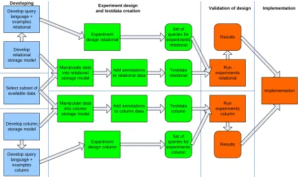
Detailed approach

This section will present the detailed approach for this research. Figure 1 shows an overview of the involved parts for this research. On the left side there are sensor stations (which contain sensors) or ‘simple’ sensors. The data will have to be collected, annotated and stored

somehow. The main focus for this research will be on the storage and retrieval parts. We assume there is a data set available and therefore we don’t need to worry about data

collection. Because our storage model will most likely be different from the original one, the data will have to be manipulated into the new format. The original data will not contain annotations and therefore they will have to be added. After the retrieval some form of display is necessary to show the results.

Figure 1: Overview of involved parts

For the storage part the plan is to use both a relational and a column database. For both database types a storage model will have to be developed for the storage of sensor data and annotations. They will also both need a retrieval component. This retrieval component should have support for querying on annotations, sensor data and both in combination with time constraints.

Figure 2 shows the detailed action plan for this research. At first the storage models for both relational and column will have to be developed and also the query languages that will be used to retrieve data again. Besides that a subset of the available data will have to be chosen. Once these steps are done the chosen data can be manipulated to fit in both storage models. Because there are no annotations yet these will have to be added to the data. Also an experiment design will have to be made describing what will exactly be done during the experiments. This should give as a result a set of queries to use in the experiments. Once all these steps are done the actual experiments can be done. If the results are not as hoped, it is possible to develop another storage model and go through the procedure again if time allows.

Finally the best solution found during the experiments will be implemented and tested again on scalability. The implementation should be usable by users and have some form of display.

Develop column storage model

Develop relational storage model

Select subset of available data Develop query language + examples column Develop query language + examples relational Manipulate data into relational storage model Add annotations to relational data

Manipulate data into column storage model

Add annotations to column data

Experiment design column Set of queries for experiments column Run experiments relational Results Testdata relational Testdata column

Validation of design Experiment design

and testdata creation

Experiment design relational Set of queries for experiments relational Developing Run experiments column Results Implementation Implementation

5.

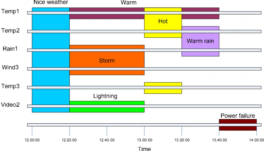
Case

This section will describe a case to show the complexity of sensor data and its annotations and to provide material to base further examples on. In the IJkdijk project [IJk09] one of the sensor stations used is a weather station which contains multiple sensors. In this case we will use this weather station as an example.

Imagine we have 3 of these weather stations with each a number of sensors. We will assume all 3 stations have the same sensors, namely a temperature sensor, a rainfall sensor, a wind speed sensor and a video camera. As we have seen in the section ‘Annotation and query types’ on page 8, annotations can be a lot more than simply be attached to a single measurement. Figure 3 shows a time span of data measurements for 6 sensors from the 3 weather stations and the following types of annotations (on sensor level) on this sensor data:

- Annotations over multiple sensor types (e.g. Warm rain) - Annotations over multiple sensor stations (e.g. Hot)

- Annotations over multiple sensor types and -stations (e.g. Storm, Nice weather, Warm rain) - Annotations over 1 sensor (e.g. Warm, Lightning)

- Annotations overlapping in time (e.g. Warm, Storm and Lightning) - Annotations on time itself (e.g. Power failure)

Figure 3: Examples of annotations over sensor data

6.

Storage of sensor data and annotations

In related work (chapter 3) we have found a number of systems and methods to store sensor data and its annotations. In this section we will discuss these methods more in detail. We will start by taking a look at the relational part and then at the column database part. For relational we will first look at a number of methods for storing sensor data and annotations. After that we will take a look at the systems found and discuss their methods used. For all methods we will discuss their advantages and disadvantages.

6.1.

Relational storage

In chapter 2 we already mentioned the simple approach of attaching annotations to

measurements and the theoretic solution of using N1NF schemas. The first was inefficient due to duplication of data when multiple annotations are attached to a single measurement. The second option is an interesting theoretic solution, but there are no databases supporting this form. Using the 1NF, a lot of redundant data is created and when querying a lot of joins have to be done, making this solution both inefficient on storage and retrieval terms.

Next we will take a closer look at the storage solutions in [WHB08]. In their opinion sensor data and annotation data are different and therefore require different storage models. Sensor data most likely consists of a timestamp, value and some sensorID. A sensor station can contain multiple sensors with different measurement types (e.g. wind speed, temperature, rainfall or video). Annotation data consists of an annotation and possibly a comment on it and it has to be related to a measurement or multiple measurements. We will first take a look at sensor data storage.

6.1.1. Sensor data storage

A few options [WHB08-2] mentioned are storing measurements per measurement type (see Table3), per sensorID (see Table 4) or all data in one big table (see Table 5). All have their advantages and disadvantages which we will discuss next.

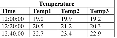
Table3 provides the advantage of efficient search for a specific measurement type like temperature. It also prevents empty cells coming from different measuring frequencies of different measurement types. Disadvantages are redundant storage of timestamps, inefficient retrieval of all measurement types or data at a certain timestamp or time space from 1 sensor and sensors must be synchronized.

Temperature

Time Temp1 Temp2 Temp3

12:00:00 19.0 19.9 19.2 12:20:00 20.5 21.2 20.3 12:40:00 22.7 23.4 22.9

Table 3: Example of sensor data storage per measurement type

Weatherstation1

Time Wind speed Temperature Rainfall

12:00:00 2.0 19.0 0.0

12:20:00 8.0 20.5 0.4

12:40:00 10.0 22.7 0.5

Table 4: Example of sensor data storage per sensor

Table 5 has the advantage of no redundant storage of timestamps and provides efficient search for all sensor data on a certain timestamp or time space. Disadvantages are that sensors must be synchronized and different frequencies create a lot of empty cells. Also scalability is low because new sensors will always introduce new columns.

Data

Time Wind1 Wind2 Wind3 Temp1 Temp2 Temp3 Rain1 Rain2 Rain3

12:00:00 2.0 3.0 1.0 19.0 19.9 19.2 0.0 0.0 0.0 12:20:00 8.0 9.0 7.0 20.5 21.2 20.3 0.4 0.5 0.4 12:40:00 10.0 7.0 9.0 22.7 23.4 22.9 0.5 0.4 0.4 Table 5: Example of sensor data storage with all data in 1 table

6.1.2. Annotation storage

There are many possible ways to store annotations. [WHB08] describes 3 types of storage that use the annotation name as table. The first uses a {time,sensor_id} tuple, the second a {time, sensor_1, sensor_2, sensor_3} tuple and the third a {start_time, end_time, sensor_id} tuple. All have their advantages and disadvantages in terms of space and search efficiency.

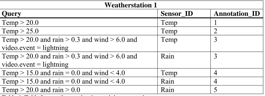
A fourth option mentioned uses a table per sensor station and {query, sensor_id,

annotation_id} tuples in it (see Table 6). Annotation_id refers to an ID in an Annotation table (Table 7) which contains all annotations for that ID and possibly a comment on it which is stored in the table Comments (see Table 8). The query returns all measurements to which the annotation applies. When searching for all measurements with a certain annotation set, the DBMS can union the queries found in that set. This type of storage also allows annotations to change name and the use of multiple annotations on a certain time interval on a sensor. If a specific time interval is requested, this can be appended to the queries as another constraint, removing the need for post-processing. Disadvantages are that storage requirements will be high if annotations are spread over small time intervals and overlapping annotations create a whole new problem for both storage and retrieval.

Weatherstation 1

Query Sensor_ID Annotation_ID

Temp > 20.0 Temp 1

Temp > 25.0 Temp 2

Temp > 20.0 and rain > 0.3 and wind > 6.0 and video.event = lightning

Temp 3

Temp > 20.0 and rain > 0.3 and wind > 6.0 and video.event = lightning

Rain 3

Annotations

Annotation_ID Value

1 {warm} 2 {hot)

3 {storm, lightning, warm}

4 {nice weather}

5 {warm rain}

Table 7: Table for storing annotation sets

Comments

Annotation_ID Comment

1 Warm outside

3 Lightning visible

4 No clouds in the sky

5 Warm rain manually

confirmed

Table 8: Table for storing additional information about annotations

6.1.3. Storage systems

The previous two sections showed ways of storing sensor and annotation data. This section will take a look at some complete systems which were also discussed in chapter 3.1. Here we will focus on how they actually store the sensor and annotation data.

MAAS

The MAAS [KMP09] system stores both sensor stations and sensors in their own table. The sensor table is linked to a station and will contain all data produced by that sensor. The ‘SensorAnnotation’ table links sensor data to an annotation. Text can be added to describe a specific annotation instance. Time ranges are supported by using aggregation of data. This method of storage produces a lot of joins in the queries. Possible existing data will have to be converted into the used format in order to use this system.

DBNotes

DBnotes [CCV05] produces extra tables in order to store the annotations. Further it uses an extension of SQL called pSQL. It does not affect the original sensor data. Experiments showed that pSQL query execution time was a factor 1 to 2 slower than normal SQL query execution time. The gain is the ability to propagate annotations.

Mondrian

BDBMS

BDBMS [EAE09] does not affect the original sensor data. Every data table can have multiple annotation tables. These tables store the annotated data using rectangles. The rectangles are built by numbering both rows and columns. In order to be truly effective, columns with a high correlation need to be next to each other. This is done using an algorithm based on statistics about the annotations present in a table. Their solution achieves more than an order-of-magnitude reduction in storage and up to 70% reduction in the queries execution time.

6.2.

Column database storage

There were no systems or methods found that are able to store and retrieve sensor data and its annotations using a column database. Therefore we will have to think of a storage method ourselves and we have chosen to do this using Google Bigtable because of its built-in time support. Since it will not be possible to use the actual Google Bigtable system, open-source alternatives will have to be used. Unfortunately these open-source alternatives are still young and have limited functionality. For example they only support the String type and do not support joins of tables.

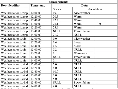
Next we will describe a solution using a ‘Bigtable’ system. Both the sensor data and the annotations will be stored in the same column family (called ‘data’) and ‘Bigtable’ provides the version management. The data will be stored under the column qualifier ‘sensor’ and the annotations under the column qualifier ‘annotation’. When multiple annotations have to be stored at a specific timestamp this works as long as they are not exactly the same.

Measurements

Row identifier Timestamp Data

Sensor Annotation

Weatherstation1.temp 12:00:00 19.0 Nice weather

Weatherstation1.temp 12:20:00 20.5 Warm

Weatherstation1.temp 12:40:00 22.7 Warm

Weatherstation1.temp 13:00:00 25.1 Warm Hot

Weatherstation1.temp 13:20:00 23.6 Warm

Weatherstation1.temp 13:40:00 NULL Power failure

Weatherstation1.temp 14:00:00 21.9 NULL

Weatherstation1.rain 12:00:00 0.0 Nice weather Weatherstation1.rain 12:20:00 0.4 Storm

Weatherstation1.rain 12:40:00 0.5 Storm Weatherstation1.rain 13:00:00 0.2 NULL Weatherstation1.rain 13:20:00 0.1 Warm rain

Weatherstation1.rain 13:40:00 NULL Power failure Weatherstation1.rain 14:00:00 0.1 NULL

Weatherstation1.wind 12:00:00 2.0 NULL

Weatherstation1.wind 12:20:00 8.0 NULL

Weatherstation1.wind 12:40:00 10.0 NULL

Weatherstation1.wind 13:00:00 6.0 NULL

Weatherstation1.wind 13:20:00 5.0 NULL

Weatherstation1.wind 13:40:00 NULL Power failure

Table 9 shows an example of what this storage will look like. Multiple sensor stations should be put into the same table in order to overcome the lack of joins. Table 10 shows what the table will look like at a specific time with all 3 weather stations in it, in this case at 12:00:00.

Measurements

Row identifier Data

Sensor Annotation

Weatherstation1.temp 19.0 Nice weather

Weatherstation1.rain 0.0 Nice weather

Weatherstation1.wind 2.0 NULL

Weatherstation2.temp 19.9 Nice weather

Weatherstation2.rain 0.0 NULL

Weatherstation2.wind 3.0 NULL

Weatherstation3.temp 19.2 Nice weather

Weatherstation3.rain 0.0 NULL

Weatherstation3.wind 1.0 Nice weather

Table 10: Example of sensor data and annotations in a 'Bigtable' system at one specific time

This storage model is able to store annotations on a row and supports time. Further it should be able to support all types of queries, although some extra logic will be necessary.

6.3.

Storage models to be used in scalability experiments

Because time is limited, we will have to make a selection of storage models to be used in our experiments. One of our goals was to use at least 1 non-relational method. Further we will choose 2 relational methods from the found ones. These models will be tested using experiments which will be discussed later on.

6.3.1. Relational storage

Considering relational storage we have chosen for the WHB08 [WHB08] and the BDBMS [EAE09] storage models. Looking at Table 1 and Table 2 we can see BDBMS has the most support for storing and querying annotations. WHB08 uses a different approach to storing annotations and we are curious what its scalability is. With WHB08 we will store sensor data per sensor station and use their 4th annotation storage option as described in the section ‘Annotation storage’ on page 19. For BDBMS extra logic will be needed to work with the annotation rectangles. We will leave out the algorithm to arrange the columns as efficient as possible and do this manually.

6.3.2. Column database storage

7.

Retrieval of sensor data and annotations

This section will describe the retrieval part of the system. We will start with looking at what kinds of retrieval are desired. Next we will give a metasyntax description of our proposed query language and we will take a look at how to convert our language into SQL and HQL.

7.1.

Types of queries

At first we will have to take a look at what types of queries should be supported in the

retrieval. In chapter 2.1 we mentioned a few types. Of these types we like to have support for:

- Querying for sensor data, annotations and time (in SELECT)

- Creating constraints on sensor data, annotations and time (in WHERE) - Combinations of above mentioned types

- Sensor data can be ‘simple’ (1 type, 1 station), multiple types, multiple stations and both - Annotation management, create, add, delete and remove annotations

7.2.

Proposed query language

Next we will define the query language that will be used to retrieve the sensor data and annotations from the storage. It is inspired by chapter 4.1 from [KMP09]. The metasyntax description of the language is the following:

query = GET TIME? ANNOTATION? “<sensor_data>” FROM “<station>” (, “<station>”)* where

| ADD ANNOTATION “<annotation>” TO “<sensor_data>” AT “<station>” where

| REMOVE ANNOTATION “<value>” FROM “<sensor_data>” AT “<station>”

| CREATE ANNOTATION “<value>” | DELETE ANNOTATION “<value>” ;

where = WHERE constraint ((AND | OR) constraint)* ;

constraint = (“<sensor_data>” | ANNOTATION | TIME ) NOT? BETWEEN “<value>” AND “<value>”

| (“<sensor_data>” | ANNOTATION | TIME ) NOT? (> | < | >= | <= | =, <>) “<value>” ;

Which should support all types of queries as mentioned in the above section. Examples can be found in the section ‘Query set for validation’ on page 27.

7.3.

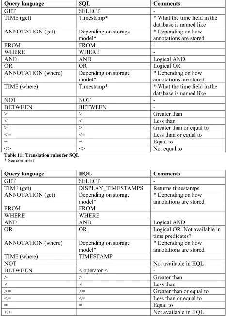
Translation rules

Query language SQL Comments

GET SELECT -

TIME (get) Timestamp* * What the time field in the database is named like ANNOTATION (get) Depending on storage

model*

* Depending on how annotations are stored FROM FROM - WHERE WHERE -

AND AND Logical AND

OR OR Logical OR

ANNOTATION (where) Depending on storage

model* * Depending on how annotations are stored TIME (where) Timestamp* * What the time field in the

database is named like NOT NOT - BETWEEN BETWEEN -

> > Greater than

< < Less than

>= >= Greater than or equal to

<= <= Less than or equal to

= = Equal to

<> <> Not equal to

Table 11: Translation rules for SQL * See comment

Query language HQL Comments

GET SELECT -

TIME (get) DISPLAY_TIMESTAMPS Returns timestamps ANNOTATION (get) Depending on storage

model*

* Depending on how annotations are stored FROM FROM - WHERE WHERE

AND AND Logical AND

OR OR Logical OR. Not available in

time predicates? ANNOTATION (where) Depending on storage

model*

* Depending on how annotations are stored

TIME (where) TIMESTAMP -

NOT Not available in HQL

BETWEEN < operator < -

> > Greater than

< < Less than

>= >= Greater than or equal to

<= <= Less than or equal to

= = Equal to

<> Not available in HQL

8.

Scalability testing of storage models

This section will describe the design of an experiment to validate possible storage methods for sensor data and its annotations. For this experiment we will use a subset of the data as

produced in IJkdijk [IJk09] experiments and provided by TNO-ICT (part of ‘Stichting IJkdijk’) to be used in this research. We will start with discussing what parts of the dataset will be used and how we will convert this data into its new storage models. Next we will present a query set which will be used to validate and compare storage models. We will describe what exactly will be tested during the experiments and finally we will present and discuss the results.

8.1.

Data set for scalability testing of storage models

TNO-ICT has provided a dataset to be used in this research. This relational dataset contains a part of the sensor measurements from the 2009 IJkdijk experiments. It has a total of

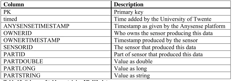
48.524.227 rows. The schema of the table containing this data is as seen in Table 13. The timestamps are the number of milliseconds passed since January 1st 1970.

Column Description

PK Primary key

timed Time added by the University of Twente ANYSENSETIMESTAMP Timestamp as given by the Anysense platform OWNERID Who owns the sensor producing this data OWNERTIMESTAMP Timestamp produced by the sensor SENSORID The sensor that produced this data PARTID Part of sensor that produced this data

PARTDOUBLE Value as double

PARTLONG Value as long

PARTSTRING Value as string

Table 13: Schema of table containing IJkdijk data

We will select a part of this data to work with. We want to use different sensor stations with multiple sensors/parts. The weatherstation sensor contains 13 parts and a total of 81.046 rows. The luisterbuis sensor (an audio sensor that also measures pressure and temperature) has 4 parts and 1.719.426 rows. We will use these 2 together as our dataset for the experiments. This makes a total of 1.800.472 rows.

8.1.1. Data manipulation

‘Appendix A: Data manipulation details’ will give more details about the manipulation process including the actual queries used. We will start storing our selected subset into a new table with the exact same schema. Next we create tables for the weather station and the luisterbuis sensor.

After taking a look at the data it seems there is erroneous data. The weather station

The luisterbuis data also contains some erroneous data. 168 measurements contain more than 4 parts and once again this is duplicate data at the same timestamp. 529 measurements contain less than 4 parts. We will again leave this data in. This makes a total of 1.768.609 rows.

The actual manipulation from the subset table to the sensor station specific tables will be done using PHP. A script will query all data for a sensor station and extract the values for all

partid’s of a single measurement. This measurement will then be inserted again into the new table. Missing parts will be inserted as nulls. In the case of Hypertable the luisterbuis and weatherstation tables were used and each column was inserted as a row with the

ownertimestamp as timestamp.

For relational data the manipulation resulted in 3.831 rows in the weatherstation table and 429.986 rows in the luisterbuis table. This makes a total of 433.817 rows. For Hypertable it was 49.803 rows for the weatherstation and 279.276 for the luisterbuis making a total of 329.079 rows.

8.1.2. Adding annotations

Next we will have to add annotations to the data. We will start creating the tables necessary for storing them. ‘Appendix B: Annotation adding details’ describes the actual queries used. For the [WHB08] method, both the weather station and luisterbuis get a table for their

annotations. Further we create the actually annotation table and a comments table. In the case of BDBMS each sensor station also gets an annotation table, but no additional tables are needed.

We will add all annotations from the case, except for lightning and power failure, to both storage models. Further we added 3 annotations for the luisterbuis data. For [WHB08] this means adding the annotations and attaching them to data using a query. For BDBMS this means creating rectangles, which will be done automated. The manually chosen column mapping for weatherstation is as follows: PK=1, OWNERTIMESTAMP=2,

WINDSPEEDAVG=3, TEMPAVG=4 and RAINFALLTOTAL=5. For luisterbuis this is: PRESSUREA=1, PRESSUREB=2, TEMPA=3, TEMPB=4. The other columns are not used in our annotations.

The results were that WHB08 got 530, 15.825 and 158.385 annotated for respectively the weatherstation, luisterbuissubset and luisterbuis. For BDBMS the number were 125, 7.649 and 76.356 rows containing rectangles.

For Hypertable we can only attach annotations to a specific sensor. For the weatherstation we will add the annotations ‘hot’, ‘warm’ and ‘cold’ to the ‘tempavg’ sensor. Further we will add ‘heavy rain’ (rain > 0.3) and ‘storm’ (wind > 6) to the ‘rainfalltotal’ and the ‘windspeedavg’ sensors. Together they form the original ‘storm’ annotation from our case. The luisterbuis will receive the same annotations as the relational luisterbuis data.

8.2.

Query set for validation

In order to test and validate the storage model, we will need a query set. This set of queries should represent the majority of possible queries over our data. Section 7.1 presented an overview of what types of queries should be supported in the query language. That list is the basis of the query set.

For our experiments we will manually translate the queries from our language to SQL for both WHB08 and BDBMS and to HQL for Hypertable. Some translations will need extra logic to produce the desired result.

Query 1, create an annotation (annotation management):

CREATE ANNOTATION 'cold';

WHB08:

INSERT INTO annotations(TIME, VALUE) VALUES(unix_timestamp(now()), 'cold');

BDBMS and Hypertable:

There are no separate tables for annotations in BDBMS and Hypertable.

Query 2, delete an annotation (annotation management):

DELETE ANNOTATION 'cold';

WHB08:

DELETE FROM annotations WHERE STRCMP(VALUE, 'cold');

BDBMS and Hypertable:

There are no separate tables for annotations in BDBMS and Hypertable.

Query 3, add an annotation to data (annotation management):

ADD ANNOTATION 'cold' TO 'weatherstation' AT 'tempavg' WHERE tempavg < 5;

WHB08:

SELECT * FROM annotations WHERE STRCMP(value, 'cold') = 0;

If not existing yet:

INSERT INTO annotations(TIME, VALUE) VALUES(unix_timestamp(now()), 'cold');

Always execute:

BDBMS:

BDBMS will have to select all rows with tempavg < 5, create rectangles of them and then:

INSERT INTO weatherstationannot2(annotationid, time, value, rectangle) values('6', unix_timestamp(now()), 'cold', ' ((4,3749),(4,3777))');

For each rectangle created.

Hypertable:

Select all data from the sensor we want to annotate:

SELECT * FROM weatherstationd WHERE

cell='weatherstation1.tempavg','timeline:base';

If it meets the annotation condition, insert the annotation into the column ‘timeline:annotation’ at the timestamp of the data.

Query 4, remove annotation (annotation management):

REMOVE ANNOTATION 'cold' FROM 'tempavg' AT 'weatherstation';

WHB08:

DELETE FROM weatherstationannot WHERE STRCMP(SENSORID, 'tempavg') = 0 AND ANNOTATIONID IN (SELECT ANNOTATIONID FROM annotations WHERE STRCMP(VALUE, 'cold') = 0);

BDBMS:

DELETE FROM weatherstationannot2 WHERE STRCMP(VALUE, 'cold') = 0;

Advanced logic is necessary to delete the annotation only from the 'tempavg' column.

Hypertable:

Because in Hypertable a delete will not only delete the data at the given timestamp, but also all earlier timestamps of that cell, only 1 delete query will delete all annotations. This is already very

impractical, but after a delete it is also not possible to immediately insert the same data again, making it even harder to test this aspect of Hypertable. Our solution is to add a unique annotation each time with query 3, then delete that one again with this query and start over with a new unique annotation. The delete will be done the following way:

SELECT * FROM weatherstationd WHERE

cell='weatherstation1.tempavg','timeline:annotation';

Then check if the value = ‘cold’ and using that timestamp execute:

Query 5, get ‘simple’ data with sensor data constraint (select ‘simple’ + data constraint):

GET tempavg FROM weatherstation WHERE tempavg > 10;

WHB08 and BDBMS:

SELECT tempavg FROM weatherstation WHERE tempavg > 10;

Hypertable:

SELECT * FROM weatherstationd WHERE cell='weatherstation1.tempavg', timeline.base';

Then filter all resulting cells with value > 10;

Query 6, get sensor data with time and annotations with sensor data constraint (select ‘simple’ and annotations + data constraint):

GET TIME ANNOTATION tempavg FROM weatherstation WHERE tempavg > 25;

WHB08:

At first all queries attached to tempavg will be selected and looped through:

SELECT query, annotationid FROM weatherstationannot WHERE STRCMP('tempavg', sensorid) = 0;

Next we will execute the following query with the query column of the result of the first query attached:

SELECT ownertimestamp, tempavg FROM weatherstation WHERE tempavg > 25 AND {query};

If this query produces at least 1 result, we will get the annotation using:

SELECT value FROM annotations WHERE annotationid = {annotationid};

Where {annotationid} is the id of the annotation as returned by the first query.

BDBMS:

SELECT ownertimestamp, tempavg FROM weatherstation WHERE tempavg > 25;

For these rows it must be checked whether they are inside a rectangle and attach the annotation(s) to the result.

Hypertable:

SELECT * FROM weatherstationd WHERE

cell='weatherstation1.tempavg','timeline:base';

Query 7, get time and sensor data consisting of multiple parts with annotation constraint (select multiple sensors + annotation constraint):

GET TIME tempavg, tempmax, tempmin FROM weatherstation WHERE ANNOTATION = 'hot';

WHB08:

SELECT a.value, wa.query FROM weatherstationannot as wa, annotations as a WHERE STRCMP(wa.query, 'tempavg > 25') = 0 AND wa.annotationid =

a.annotationid;

SELECT ownertimestamp, tempavg, tempmax, tempmin FROM weatherstation as w, weatherstationannot = wa WHERE w.{result->wa.query};

BDBMS:

SELECT rectangle FROM weatherstationannot2 WHERE STRCMP(value, 'hot') = 0;

The rectangle(s) have to be converted to rows and colums and then we query:

SELECT ownertimestamp, tempavg, tempmax, tempmin FROM weatherstation WHERE pk = row(s);

Hypertable:

SELECT * FROM weatherstationd WHERE

cell='weatherstation1.tempavg','timeline:annotation' and cell='weatherstation1.tempmax','timeline:annotation' and cell='weatherstation1.tempmin','timeline:annotation';

Compare with ‘hot’ and if it matches, get data at that timestamp.

Query 8, get time and sensor data with time constraint (select ‘simple’ + time constraint):

GET TIME tempavg FROM weatherstation WHERE TIME BETWEEN '1253358800000' AND '1253369970000';

WHB08 and BDBMS:

SELECT ownertimestamp, tempavg FROM weatherstation WHERE ownertimestamp BETWEEN '1253358800000' AND '1253369970000';

Hypertable:

SELECT * FROM weatherstationd WHERE

Query 9, get annotations, time and sensor data in a certain time range (select ‘simple’ and annotations + time constraint):

GET TIME ANNOTATION tempavg FROM weatherstation WHERE TIME BETWEEN '1253358800000' AND '1253369970000';

WHB08:

First we select the queries and values of all annotations and loop through them:

SELECT wa.query as q, a.value as v FROM weatherstationannot as wa, annotations as a WHERE wa.annotationid = a.annotationid;

Next we execute the following query where {query} comes from the result of the first query:

SELECT pk, ownertimestamp FROM weatherstation WHERE {query} AND ownertimestamp BETWEEN '1253358800000' AND '1253369970000';

And then we can display all data with that annotation within the given time range.

BDBMS:

For BDBMS the rows from weatherstation will have to be selected and then check if the row numbers are inside a rectangle.

Hypertable:

SELECT * FROM weatherstationd WHERE

cell='weatherstation1.tempavg','timeline:base' AND '2009-09-19 13:13:20' < TIMESTAMP < '2009-09-19 16:19:30';

Loop through data and query annotations at the same timestamp as the data.

Query 10, get time and sensor data from multiple stations (select multiple stations):

GET TIME tempavg, tempa FROM weatherstation, luisterbuis WHERE tempavg = tempa;

WHB08 and BDBMS:

SELECT w.ownertimestamp, tempavg, l.ownertimestamp, tempa FROM weatherstation as w, luisterbuis as l WHERE w.tempavg = l.tempa;

Hypertable:

SELECT * FROM luisterbuisd WHERE cell='luisterbuis.tempa','timeline:base'; SELECT * FROM weatherstationd WHERE

cell='weatherstation1.tempavg','timeline:base';

8.3.

Experiment design

We have selected a dataset and created a query set. Now we will define what exactly will be done. Our goal is to test the systems in terms of scalability to find out whether a data set that is 10 times larger produces query execution times that are 10 times bigger.

Most queries of [WHB08] can directly be translated to SQL, but for BDBMS this is not always possible. We will have to create some extra logic to be able to translate these queries and this will be done using PHP. We will use MySQL for the relational data. Two files were created, one for each relational storage model. Each query is put into a function and using a while loop we can execute the queries we want as many times as we want. Where necessary the MySQL query cache was emptied. The resulting average execution time per query is then outputted to the screen. Time will be measured in ‘wall clock time’, which means the total time used by the CPU, I/O and communication channels (which is equivalent to the real time passed). Further we will calculate the standard deviation for the produced results. In the case of BDBMS extra functions were created to deal with the annotation rectangles. In PHP time is measured using the ‘microtime’ function, which produces the time in microseconds.

For Hypertable we will use C++ as a programming language to directly communicate with the database. Using a program called Thrift it is possible to use other languages like PHP and Java, but this will severely impact the performance and scalability. In C++ time is measured using the ‘gettimeofday’ function, which also produces the time in microseconds.

For all systems we will try to run the 10 queries 1000 times on data set size 1, 100 times on data set size 2 and 10 times on data set size 3. This will be done because some queries will start taking a lot of time at larger data sets. More on these data set sizes can be found in the next section.

8.3.1. Data set sizes

In order to measure scalability we will have to run our tests on different scales. We can scale two things, data and annotations. In these experiments we will only scale the data, but as the data grows the annotations will grow along. The preferred data set sizes are 10.000, 100.000 and 1.000.000, but currently our dataset only consists of 433.000 tuples. For now we will use this set, but for the real scalability tests we will either receive more data from TNO or expand the data ourselves to 1 million. The three data set sizes will all get their own table. The smallest data set size will be the weatherstation data, consisting of 3.831 rows. The middle data set size will consist of a subset of the luisterbuis data (42.999 rows) and the largest data set size will be the whole luisterbuis table containing 429.986 rows. This distribution of scales means we will have to use different queries for the largest 2 data sets compared to the

smallest. These queries can be found in ‘Appendix C: Queries for larger data sets using luisterbuis’. Query 10 is only possible on the larger data sets since it involves both the weatherstation and luisterbuis data.

For Hypertable the weatherstation has 49.803 cells, the luisterbuis subset 171.996 and the luisterbuis 776.871. The numbers are larger because each sensor is a row instead of a column. The largest data set is also larger because we duplicated data in order to get a better scale.

Data set size 1 Data set size 2 Data set size 3 Rows of relational

data

3.831 42.999 429.986

Rows of WHB08 annotations

530 15.825 158.385

Rows of BDBMS annotations

125 7.649 76.356

Rows of Hypertable data

49.803 171.996 776.871

Rows of Hypertable annotations

931 54.885 276.494

Table 14: Overview of data set sizes

8.4.

Results

This section will talk about the results of the experiments for all three storage models. At first we will give the 10 queries more meaningful names than just ‘Query x’. The annotation management queries get short versions of their full names. For the selection queries this will not work and therefore we created abbreviations with the following format: ‘Query number. Select(S): Data(D)/Annotation(A)/Time(T)/Constraint on(C):

Data(D)/Annotation(A)/Time(T)’. These abbreviations show what a query selects and which constraints it has. Table 15 and Table 16 show the mapping of queries to these abbreviations.

Create_annot Delete_annot Add_annot Remove_annot

Query number 1 2 3 4

Table 15: Mapping of annotation management queries to abbreviations

CONSTRAINT ON SELECT

Data Annotations Time

Data 5, 6, 10 7 8, 9

Annotations 6 x 9

Time 6, 10 7 8, 9

Table 16: Mapping of selection queries to abbreviations

Next we will take a look at what exactly each query does. Table 17 shows this for the relational data and for all 10 queries on the 3 scales. The standard deviations for all

Query Data set size 1 Data set size 2 Data set size 3

1. Create_annot Insert 1 row Insert 1 row Insert 1 row

2. Delete_annot Delete 1 row Delete 1 row Delete 1 row

3. Add_annot Insert 1 row Insert 1 row Insert 1 row

4. Remove_annot Delete 1 row Delete 1 row Delete 1 row

5. S: D/C: D Select 3076 rows Select 29.767 rows Select 298.116 rows

6. S: DAT/C: D Select 588 rows, 3

tables involved

Select 5342 rows, 3 tables involved

Select 52.793 rows, 3 table involved

7. S: DT/C: A Select few annotation

rows + 20 rows Select few annotation rows + 61 rows Select few annotation rows + 617 rows

8. S: DT/C: T Select 304 rows Select 3169 rows Select 31687 rows

9: S: DAT/C: T Select 174 rows Select 1269 rows Select 12690 rows

10: S: DT/C: D * Select 588 rows, 2

tables involved Select 5782 rows, 2 tables involved Table 17: What each query does on every scale

8.4.1. WHB08

Table 18 and Figure 4 show the results of the experiments with WHB08 data and annotations. Query 10 was not run on data set 1 because it involves both the weatherstation and luisterbuis data and therefore is at least data set 2. The column “1<>2” shows the difference between the execution times of data sets 1 and 2. The column “2<>3” does the same for data sets 2 and 3.

Creating, inserting, deleting and removing are very scalable processes. Queries 6, 9 and 10 have a good scalability and 5, 7 and 8 a poor scalability. In general the standard deviation was low, but on scale 1 it was high, making the “1<>2” column less trustworthy. Also some measurements have such low execution times that the standard deviation becomes less relevant due to the accuracy of the measurements.

Query Data set 1 [s] 1<>2 Data set 2 [s] 2<>3 Data set 3 [s]

1. Create_annot 0.000075 1.25x 0.000094 1.21x 0.000114

2. Delete_annot 0.000085 1.22x 0.000104 1.02x 0.000106

3. Add_annot 0.000165 1.33x 0.000219 1.02x 0.000223

4. Remove_annot 0.000160 1.11x 0.000178 1.03x 0.000183

5. S: D/C: D 0.000348 14.39x 0.005006 172.20x 0.862047

6. S: DAT/C: D 0.018436 2.78x 0.051219 9.78x 0.500611

7. S: DT/C: A 0.000112 1.33x 0.000149 211.06x 0.031448

8. S: DT/C: T 0.000072 10.49x 0.000755 274.90x 0.207547

9: S: DAT/C: T 0.000479 4.31x 0.002064 15.82x 0.018178

10: S: DT/C: D * * 20.335640 8.81x 191.751825

PHP max memory 190.376

bytes

1.00x 190.376 bytes 1.00x 190.376 bytes

Table 18: Execution times and peak memory usage of queries on WHB08 in seconds and bytes * Not applicable

Execution times of queries on WHB08 in seconds on a logaritmic scale

0,00001 0,0001 0,001 0,01 0,1 1 10 100 1000 1. Create_annot

2. Delete_annot 3. Add_annot 4. Remove_annot 5. S: D/C: D 6. S: DAT/C: D 7. S: DT/C: A 8. S: DT/C: T 9: S: DAT/C: T 10: S: DT/C: D

Data set 1 0,000010 0,000479 0,000072 0,000112 0,018436 0,000348 0,000160 0,000165 0,000085 0,000075 Data set 2 20,335640 0,002064 0,000755 0,000149 0,051219 0,005006 0,000178 0,000219 0,000104 0,000094 Data set 3 191,751825 0,018178 0,207547 0,031448 0,500611 0,862047 0,000183 0,000223 0,000106 0,000114

1. Create_ann ot 2. Delete_anno t 3. Add_annot 4. Remove_an not 5. S: D/C: D 6. S: DAT/C:

D 7. S: DT/C:

A 8. S: DT/C:

T 9: S: DAT/C:

T 10: S: DT/C:

D

8.4.2. BDBMS

Table 19 and Figure 5 show the results of the experiments with BDBMS data and annotations. Query 1 and 2 were not run because BDBMS does not have the annotations separately stored, the annotations are simply linked to the data directly. Query 10 was not run on data set 1 because it involves both the weatherstation and luisterbuis data and therefore is at least data set 2. The column “1<>2” shows the difference between the execution times of data sets 1 and 2. The column “2<>3” does the same for data sets 2 and 3.

The insertion and removal of annotations for BDBMS is less scalable than WHB08, but it is still acceptable. Queries 7 and 10 are the only other queries with a good scalability. Queries 5 and 8 have a reasonable scalability and 6 and 9 a bad scalability. The absolute numbers of query 6 and 9 get very high for data set 3. The standard deviation was overall low.

Query Data set 1 [s] 1<>2 Data set 2 [s] 2<>3 Data set 3 [s]

1. Create_annot * * * * *

2. Delete_annot * * * * *

3. Add_annot 0.004724 38.85x 0.183509 11.66x 2.140202

4. Remove_annot 0.000881 38.63x 0.034033 10.27x 0.349678

5. S: D/C: D 0.000356 10.58x 0.003765 225.90x 0.850495

6. S: DAT/C: D 0.056388 983.18x 55.439357 101.60x 5632.72

7. S: DT/C: A 0.000242 315.45x 0.076339 26.22x 2.001602

8. S: DT/C: T 0.000078 7.05x 0.000550 374.74x 0.206108

9: S: DAT/C: T 0.015473 738.58x 11.428085 102.39x 1170.066720

10: S: DT/C: D * * 20.504747 9.34x 191.569171

PHP max memory 1.702.120 bytes 8.00x 13.617.968

bytes

9.67x 131.615.152 bytes Table 19: Execution times and peak memory storage of queries on BDBMS in seconds and bytes * Not applicable

Execution times of queries on BDBMS in seconds on a logaritmic scale

0,00001 0,0001 0,001 0,01 0,1 1 10 100 1000 10000 3. Add_annot

4. Remove_annot 5. S: D/C: D 6. S: DAT/C: D 7. S: DT/C: A 8. S: DT/C: T 9: S: DAT/C: T 10: S: DT/C: D

Data set 1 0,000010 0,015473 0,000078 0,000242 0,056388 0,000356 0,000881 0,004724 Data set 2 20,504747 11,428085 0,000550 0,076339 55,439357 0,003765 0,034033 0,183509 Data set 3 191,569171 1170,066720 0,206108 2,001602 5632,720000 0,850495 0,349678 2,140202 3. Add_annot 4.

Remove_annot 5. S: D/C: D

6. S: DAT/C: D 7. S: DT/C: A

8. S: DT/C: T 9: S: DAT/C: T

8.4.3. Hypertable

Table 20 and Figure 6 show the results of the experiments with Hypertable data and annotations. Query 1 and 2 were not run because Hypertable does not have the annotations separately stored, the annotations are simply linked to the data directly. Query 10 was not run on data set 1 because it involves both the weatherstation and luisterbuis data and therefore is at least data set 2