Emergent swarm morphology control of wireless networked mobile robots

Emergent Swarm Morphology Control

of Wireless Networked Mobile Robots

Julien Nembrini and Alan F.T. Winfield

Abstract We describe a new class of decentralised control algorithms that link local wireless connectivity to low-level robot motion control in order to maintain both swarm aggregation and connectivity, which we term “coher-ence”, in unbounded space. We investigate the potential of first-order and second-order connectivity information to maintain swarm coherence. For the second-order algorithm we show that a single β parameter—the number of shared neighbours that each robot tries to maintain—acts as an “adhesion” parameter. Control ofβ alone affects the global area coverage of the swarm. We then add a simple beacon sensor to each robot and show that, by creating aβ differential between illuminated and occluded robots, the swarm displays emergent global taxis towards the beacon; it also displays interesting global obstacle avoidance properties. The chapter then extends the idea of β het-erogeneity within the swarm to demonstrate variants of the algorithm that exhibit emergent concentric or linear segregation of subgroups within the swarm, or—in the presence of an external beacon—the formation of horizon-tal or vertical axial configurations. This emergent swarm morphology control is remarkable because apparently simple variations generate very different global properties. These emergent properties are interesting both because they appear to have parallels in biology, and because they could have value to a wide range of future applications in swarm robotics.

1 Introduction

This chapter investigates robot swarms that combine sensing, locomotion and morphological adaptivity. We develop wirelessly connected robots in

Julien Nembrini, Swarm-Intelligent Systems Group, EPFL, 1015 Lausanne, Switzerland, e-mail: Julien.Nembrini@epfl.ch; Alan F.T. Winfield, Bristol Robotics Laboratory, UWE Bristol, Bristol BS16 1QY, UK, e-mail: Alan.Winfield@uwe.ac.uk

which the wireless network becomes the “glue” physically connecting the robots. Previous work studied the possibility of gathering sensory data across an ad hoc wireless connected network of mobile robots with range-limited communication and was focused on randomly moving robots in a bounded space [34]. Here we extend this idea to an unbounded space, controlling the behaviour of the robots in order to form a dynamically connected stable swarm, which we call a “coherent” swarm. Working primarily in simulation, but with partial confirmation of results with real-robot experiments, we show that with only an omni-directional wireless and collision avoidance device we can achieve coherence in an unbounded environment, i.e., the swarm forms a single connected communication network. Adding a simple beacon sensor, we also demonstrate emergent directed swarming (taxis) towards a beacon, then extend our approach to allow emergentswarm morphology control.

Swarm robotics is the study of artificial or embodied systems based upon the principles of swarm intelligence [9]. In swarm robotics a number of rel-atively simple robots, each with limited sensing, cognition and actuation, collectively work together. Robotic swarms are fully distributed systems that typically exploit emergence or self-organisation, rather than direct control, to achieve an overall task [12]. Some tasks may be biologically plausible, such as cluster sorting [6], co-operative wall building [20], or collective foraging [18]. A fundamental property of robot swarms is that they are physically distributed and it follows that flocking andformation control have been the subject of much research:

• Flocking is the task of forming a group of robots when the actual shape of the group is not important, [26, 19]. When the group is formed because of mutual attraction or because the group is attracted by a common source, such as a beacon, it will be referred to asswarming. Hayes et al. introduce the idea ofsecondary swarming where individuals relay the signal of the beacon, which makes the robots move as a group [14].

• In their study of formation control, Balch and Arkin state that research on formation control can be divided into unit-center-, leader- or neighbour-referenced control [4]. In most cases, the task for these robots is to move in the same direction while trying to maintain constant relative distances. This typically involves a constrained number of robots. Relevant to this chapter is the work presented in [5] where the use of a neighbour-referenced algorithm allows for scalability. Weßnitzer et al. describe an example of formation control using wireless communication [33].

communication is able to increase efficiency [3]. The work of this chapter employs direct robot-robot communication but adopts the framework of sit-uated communication proposed by Støy: it applies when “both the physical properties of the signal that transfers the message and the content of the message contribute to its meaning” [29]. Also of relevance to our work is the field of sensor networks with mobile nodes [25].

Since this chapter involves morphology control, i.e., regarding the entire swarm as a single entity, it also concerns the field of reconfigurable robots. Such systems typically consist of elementary robots that physically assemble to form a bigger entity [17], or modular robots whose morphology can be eas-ily changed [32]. The design of reconfigurable robots raises complex problems of distributed control and communication, but the main challenge is without doubt the physical design of an individual robot. An example of distributed control of articulated modules that can be reconfigured on-the-fly can be found in [31]. The SwarmBot project considers mobile robots able to physi-cally attach to each other to behave as a single multi-robot system [21, 13]. Perhaps closest to the topic of this chapter is a swarm of physically but flexibly connected robots that demonstrate emergent swarm taxis [28].

The remainder of the text is organised as follows: Section 2 describes our experimental method, Section 3 presents the different algorithms that were developed to achieve coherence, with a study of the behaviour of the most successful one: theβ-algorithm, Section 4 develops and investigates an emer-gent taxis behaviour relying on the dynamic differentiation between robots within the swarm, Section 5 investigates the potential of static and dynamic differentiation to actually control the global shape of the swarm, and overall conclusions are drawn in Section 6.

2 Methods

The experimental approach of this work has been to design and test swarm robotic algorithms in simulation, validated—where possible—by experiments with laboratory robots. Our simulation does not attempt to model the dy-namics of the robots. We would argue that dynamical simulation is not nec-essary for modelling swarm systems in which velocities and accelerations are modest and where robots do not come into physical contact. Our simula-tion does, however, aim to model the kinematics, sensors and actuators with reasonable fidelity so that we have a valid basis for comparison between sim-ulation and real-robot experiments.

or angle turned, that they have short-range infra-red avoidance sensors with rangera, and that they are equipped with a radio device with a limited range

rw, wherera< rw.

Fig. 1 The Linuxbots at the Bristol Robotics Laboratory (BRL).

The robots’ control system, for both simulation and real-robot experi-ments, is designed as afinite state au-tomaton. A robot will be in one of sev-eral mutually exclusive states, and can switch between them according to en-vironmental cues. In this chapter the messages coming from other robots are considered as a part of the robot’s environment. The control architecture can be divided, following [11], into two layers: avoidance andcommunication. The goal of the avoidance layer is to steer the robot away from any obstacle

that it detects (in a Braitenberg fashion [10]), while the communication layer responds to messages from neighbours (as will be described in Section 3). It is important that when the robot is performing control actions dictated by the avoidance layer, it does not take account of information from the commu-nication layer. In Brooks’ terminology, the avoidance layer “subsumes” the communication layer, because of its priority for the robot’s safety. For a full account of the control architecture, see [22].

CommunicationAn idealised model is used to simulate radio communica-tion between the robots. We assume that the wireless antenna is omnidirec-tional and that the receiver is not able to detect any message if the transmitter is located further away than a distancerw, thecommunication range. We do

not attempt to simulate buffer overflow or any other real phenomena such as signal decay, and we consider that a robot can send a message to all neigh-bours within rangerw. Noise is modelled as loss of the entire message with a

constant probability. This probability was chosen to range from zero to 10% (which represents a very poor signal-to-noise ratio).

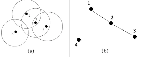
The situation depicted in Fig. 2a shows a group of robots together with each of their ranges of communication. In this example, Robot 1 can municate with Robot 2, and the latter with Robot 3. Robot 4 cannot com-municate with the other robots. This situation can be formalised using an undirected graphG= (V, E) where V is a set of points, thevertices, repre-senting the robots, and E is a set of lines, the edges, connecting one vertex to another, representing the possibility for the two robots to communicate. It is then possible to draw the graphG, hence the situation of Fig. 2a can be formalised as in Fig. 2b.

sim-(a) (b)

Fig. 2 Four numbered robots shown (a) with disks of communication ranges in 2D, and (b) as an undirected graph.

ulation, and the internal clock state of the robots is periodically randomly altered to avoid any unintended synchronicity.

3 Swarm Coherence

The goal of swarm coherence is to guarantee that the network created by the wireless connected robots of the swarm forms a single connected compo-nent, and our aim is to ensure this coherence while using minimal exchange of information. In our proposed swarm, the only relative positional infor-mation available to a robot is inferred from the interplay of the short-range avoidance behaviour and the longer, but still limited-range, wireless com-munication. Thus a robot can minimally classify the range of its neighbours according to whether they are “close” (within wireless range), “too close” (within avoidance range) or “away” (outside wireless range). We now show how the exchange of messages between the robots is critical to transform this crude data into sufficient information to achieve coherence.

Fig. 3 Basic algorithm: a robot is shown as a circle and its heading as a short line.

global time is implemented, the robots should react asynchronously. How-ever, if each robot has the same range of communication then both reactions should occur within a short time, depending on the periodicity of the calling messages. We refer to this periodicity as cadence, and we choose a default value of 100 time steps.

This behaviour leads to the two robots maintaining themselves in range as if they were attached with an elastic connection. The choice of a random heading when reconnection occurs makes the pair follow a random walk. It is important to observe that the reciprocity of reaction, even though it does not have to be simultaneous, is crucial to retaining the connection. Homogeneous robots have equal velocities and the reaction of only one robot could lead to an endless pursuit. We formally define coherence of a wireless connected swarm as follows:The swarm is considered to be coherent if any break in the overall connectivity of the network lasts less than a time constantC. Clearly, the constantCis related to the periodicity of the calling messages (cadence). In the results that follow we have chosenC = 10∗cadence; for any runs in which a break in connectivity exceedsC, the swarm is declared disconnected and the run unsuccessful. The default values of parameters for the simulation and real-robot experiments of this section are given in table 1.

Table 1 Default parameter values for swarm coherence.

αcoherenceβcoherenceβarea coverage βreal-robot

swarm size 20 or 60 20 20 7

cadence 100 100 100 100

random noise 2% 2% 2% –

αorβvalue 6 2 or 5 2 or 5 2

time steps 50,000 100,000 100,000 variable

runs 10 10 10 10

3.1 Connection degree algorithm: the

α

-algorithm

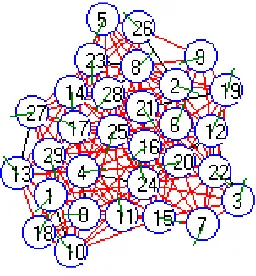
Fig. 4 30 simulated robots aiming for a complete graph.

Applying this basic algorithm to a greater number of robots by making each robot re-act to every loss of connection leads to an over-reactive swarm which clumps together (Fig. 4). To react to every loss of connection is equivalent to aiming towards a complete graph where each vertex is connected to ev-ery other, which is not our aim.

So the problem for the robot is choosing

this number falls below α. This is close to the approach adopted in Støy’s algorithm [30], although it relies on differences in the number of neighbours without the help of thresholds. Thus, in his case, while robots stay together more than random movement alone would allow, the coherence of the net-work is not assured.

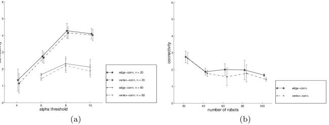
Results of α-algorithm simulation Fig. 5a shows the global degree of edge- and vertex-connectivity with increasing values of the α threshold for swarms of 20 and 60 robots. The most striking feature is the fall in connec-tivity between a swarm of 20 robots and a swarm of 60. Note that only the runs ending with a succesfully connected swarm were retained. The propor-tion of successful runs is 85% for 20 robots and 66% for 60 robots. In order to investigate more closely the drop of connectivity between swarm size, the parameterαwas also fixed to the value of 6 while the size of the swarm varied (Fig. 5b). There, the drop of connectivity can clearly be followed as the size increases. Again these results are from successful runs only.

(a) (b)

Fig. 5 Global degree of α-algorithm connectivity. (a) Increasing α under swarm sizes n= 20 (‘*’) andn= 60 (‘+’). (b) Increasing swarm size underα= 6.

(a) (b)

Fig. 6 Extreme connectivity states presenting single points of failure. (a) Examples of singular vertices, called “bridges”. (b) Example of a singular vertex, called a “cutvertex”.

Thus we have an explanation for the drop in connectivity observed: the measures of edge- and vertex-connectivity are global measures. This means that a single change in the network topology can potentially lead to a de-crease in the connectivity value. With an increasing swarm size, the prob-ability of the occurrence of such situations increases. In fact, the connec-tivity measures represent the resilience of the network to component fail-ure: the edge-connectivity value is the number of connections—regardless of which ones—that can be lost without disconnecting the network, whereas the vertex-connectivity value represents the number of nodes that can be re-moved without disconnection (a node removal will happen, for instance, in the case of a robot communication failure).

3.2 Shared neighbour algorithm: the

β

-algorithm

To avoid the extreme configurations of Fig. 6, we make use of the graph theory concept of clustering: instead of considering only its own degree of connection, each robot will receive from its neighbours their “adjacency ta-ble”, i.e., their neighbours’ lists, in order also to check whether a particular neighbour isshared, that is whether a particular neighbour is the neighbour of other robots.

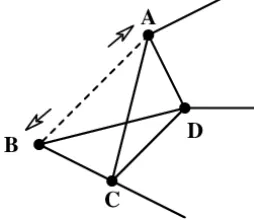
Fig. 7 Shared neighbour.

Hence Robot A will react and turn back only if the threshold β is set equal or greater than two. The algorithm tries to maintain the triangulation ob-servable in Fig. 7, therefore avoiding the extreme states. Note that Robot B may also react to the loss of connection with Robot A; this reciprocity is desirable. Pseudo-code for the β-algorithm of each robot is listed in Fig. 8.

Create list of neighbours for robot, Nlist k = number of neighbours in Nlist

i = 0

loop forever {

i = i modulo cadence

if (i = 0) { Send ID message

Save copy of k in LastK

Set reaction indicator Back to FALSE k = number of neighbours in Nlist

Create LostList comparing Nlist and OldList

for (each robot in LostList) {

Find nShared, number of shared neighbours if (nShared <= beta) {

Set reaction indicator Back to TRUE }

}

if (Back = TRUE) {

turn robot through 180 degrees }

else if (k > LastK) { make random turn }

Save copy of Nlist in Oldlist }

Steer the robot according to state Listen for calls from robots in range

Grow Nlist with neighbours IDs and connection info

i++ }

Fig. 8 Pseudo-code for theβ-algorithm.

intro-duced. However, communication remains situated, and hence message loss or misinterpretation only leads to over-reactivity without loss of robots, as the introduction of noise into the simulation confirms. Furthermore, the increase in bandwidth does not affect the scalability of the algorithm as it concerns only exchanges between neighbouring robots; messages are not propagated beyond more than a single hop in the network.

IfM is the maximum number of neighbours, then the length of a transmit-ted message will not be greater than M2_{robot identification numbers (IDs)}

(M neighbours each with M neighbours). An approximation forM is given as follows:

M =lAcomm Abody

m

−1

where Acomm is the robot’s communication area, Abody is the area of the

robot’s body andd.eis the upper rounded integer function.

It is worth stressing that the significant benefits gained from the increase of information exchange needed by theβ-algorithm could not be achieved in the framework of theα-algorithm. Thesecond-order information, about the neighbours of a neighbour, is crucial to detect bridges and cutvertices before they form. This follows from the fact that the first-order information of one robot connected to another is not sufficient to determine the nature of this connection in terms of the connectivity of the neighbouring network.

3.2.1 β-algorithm simulation results

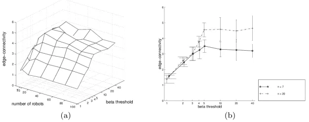
Fig. 9 shows the variation of the edge-connectivity with an increase in β threshold and swarm size. The drop in connectivity observed in the results of theα-algorithm is no longer seen. With theβ-algorithm, in contrast, con-nectivity is more constant against swarm size increase. Fig. 9a also shows that the connectivity increases sharply with increasingβ, then levels out at β values between 5 and 10.

(a) (b)

The reason for this leveling is due both to the avoidance behaviour that comes into action when robots are close together, and the fact that with high values of β, aggregation takes some time to complete. The typical mid-run configuration is a highly connected swarm with a few satellite robots that need some time to aggregate with the rest of the swarm. Because of the global nature of the connectivity measure these satellites can lead to a slight underestimate of the connectivity, which we would not observe with much longer runs. Also, smaller swarms seem to present a slightly lower perfor-mance, especially with higher values of β. The reason is the higher dynam-icity of smaller swarms that gives them a more brittle behaviour (Fig. 9b). The vertex-connectivity measure, almost equal to the edge-connectivity, is not shown for readability.

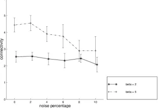
Fig. 10 Edge-connectivity against noise in theβ-algorithm withn= 20.

We now test the β-algorithm with increasing levels of noise, and the re-sults are shown in Fig. 10. Note that this curve has been obtained with in-creasing levels of noise in communica-tion, proximity sensors and actuators simultaneously. This is by no mean re-alistic, as there is no reason that the amount of noise in actuators should be proportional to communication noise. It does, however, provide a worst case evaluation of the effect of noise. A drop in connectivity with increasing noise

can be observed, but it is small in the case ofβ= 2.

The introduction of noise directly decreases connectivity due to the loss of messages. With increasing noise, a robot experiences more disconnection and as a result its reactivity increases, which maintains the connectivity for β = 2 (Fig. 10). With a higher threshold value β = 5, a swarm is more reactive, hence the potential to absorb the decrease of connectivity due to noise is lower, and the expected drop in connectivity at higher noise is clearer.

(a) (b)

Fig. 11 Examples of area coverage with (a)β= 1 and (b)β= 4.

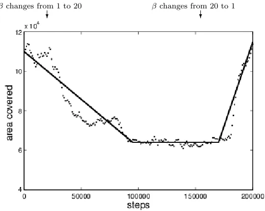
Fig. 12 shows the area covered by a swarm of 40 robots when theβ thresh-old is stepped fromβ= 1 toβ= 20 and vice-versa, which confirms that the threshold value can indeed be used to control the area coverage. It is also interesting to note that swarm spreading is much faster than swarm aggre-gation: when β is raised, the area coverage is slowly reduced to reach an equilibrium in around 100,000 time steps, whereas the swarm only needs about one quarter of this time to return to its initial area.

βchanges from 1 to 20

?

βchanges from 20 to 1

?

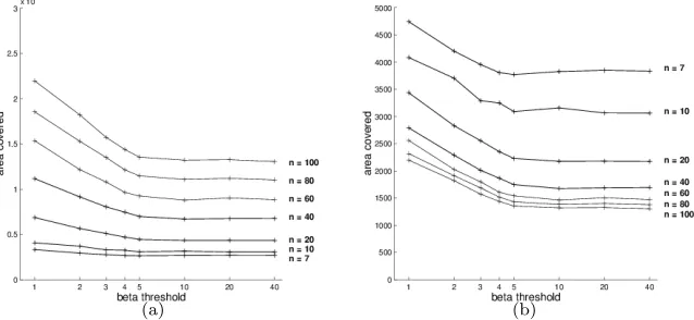
When the mean area covered by the swarm is plotted againstβfor different swarm sizes, we obtain the family of curves of Fig. 13a. Here, the potential of the β threshold to control the area is clear, and control is effective up to a value of β = 10. Beyond this value, the contraction of the swarm takes longer than the length of the run, and is therefore not measured. But in any case, the contraction is limited firstly by the low-level avoidance behaviour and secondly by the physical size of the robot body. What is also significant is the linear increase of the area when increasing the size of the swarm. This increase can also be modulated by theβ threshold without compromising its linearity. This shows that there is no leveling of the action of the algorithm and we can therefore potentially control the area ofany swarm size.

(a) (b)

Fig. 13 Area coverage againstβand swarm size (a) absolute area (b) normalised area.

The swarm area divided by the number of robots gives the mean con-tribution of a single robot to the coverage (Fig. 13b). For all swarm sizes, the slope of the decreasing normalised area is strikingly similar. This confirms that the effectiveness of theβ-control is independent of the number of robots. Of course, the effect on the whole swarm area is greater with larger swarms (Fig. 13a). The decrease of the contribution for increasing swarm sizes is due to overlapping communication areas: for larger swarms, a greater proportion of robots are situated within the swarm. Because of overlaps, these robots do not contribute as much as robots at the boundary to the whole swarm area. As expected, this decrease levels out with increasing swarm size.

Fig. 14 Area coverage vs. noise.

forβ= 5. The increase corresponds to a drop in connectivity which suggests that an increase in noise could lead to a more brittle swarm. Nevertheless the fact that the area shows such a small variation with a large increase in noise is a clear strength of the algorithm.

3.2.2 Real-robot experiments

Experimental detailsThe Linuxbots are equipped with an IEEE 802.11b wireless LAN device for TCP/IP communication both to allow robots to be started, stopped and monitored from fixed workstations, and for direct robot-robot wireless communication, as described in [36]. However, the WLAN de-vice has a range of a few hundred metres. A much shorter range of the order of one metre is required. We therefore simulate this requirement by measuring distances between robots using the robots’ infra-red (IR) tower and allowing them to communicate only if within range, a method referred to as virtual sensing [7]. The IR tower consists of a circular array of eight IR emitters under a circular array of IR receivers. In order to maintain the same ratio between avoidance range and communication range as in the simulation, the robots were calibrated with a range distance of 1.2 metres. The IR tower used is actually very noisy and the resulting virtual sensor does not corre-spond exactly with the idealised model of the simulation (see Section 2). In particular, the IR signal is not omnidirectional as the range is different in asymmetrical directions around the robot, resulting in a non-circular area of communication.

The Linuxbots’ obstacle avoidance IR sensors are situated as follows: two mounted symmetrically at the front and one at the rear, each with a range of approximately 50cm. In all real-robot experiments the physical environment is a 9-metre wide powered-floor octagon delimited by white edges suitable for IR reflection. Each experiment starts with the robots randomly grouped near the centre of the arena and lasts until the group is obviously disconnected. This approach was necessary because of the restricted size of the arena which, if permitted, would allow a lost robot to return to the swarm by reflecting back from the arena boundary, thus negating the basic assumption of an unbounded environment.

Each measured quantity was recorded every time a message was sent and has been averaged over the whole run. For a number of values of swarm size, β, and cadence, an average of 10 runs have been performed and the result given is the mean over these runs with its standard deviation. Unless varied, the default values for the remaining parameters are as shown in Table 1.

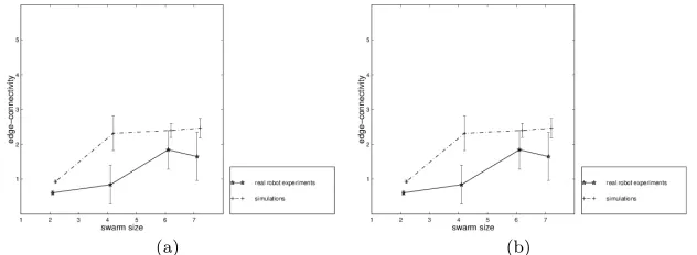
the real-robot experiments does not differ significantly from that observed in simulation (see Fig. 17 for pictures of 7 robots running theβ-algorithm).

Investigating the performance of theβ-algorithm with different real-robot swarm sizesm, we obtain Fig. 15. A much lower connectivity than in the simu-lation with a swarm of 7 robots is observed, even in the presence of 10% noise. However, the length of the runs is much shorter: in simulation, the runs were arbitrarily stopped after some time, while the real-robot experiments were halted because of robots disconnecting themselves from the swarm (typically after 2 minutes). The number of exchanged messages was 1000 in a successful simulation run and only 35 for the average length of a real-robot run. As a result, theβ-algorithm has not been definitively proven to lead to swarm co-herence on the experimental platform that was used. Note that measurement of connectivity presents some difficulties: as the real robots are asynchronous finite-state real machines, there is no global “clock” to allow for a meaningful sample of the topology of the network. The measures were recorded on board each robot, but the inevitable drift between the robots’ processing cycles weakens the accuracy of the connectivity measure.

(a) (b)

Fig. 15 Edge-connectivity inβ-algorithm real-robot experiments vs. simulation, as a func-tion of (a) swarm size, and (b)βvalue.

In fact, the lower connectivity observed in real-robot experiments is not, as one might expect, due to the difference between the non-ideal IR-tower virtual communication and the idealised communication model of the simu-lation. It is largely due to interference between the short-range IR avoidance sensors, which operate on the same frequency. This interference triggers a proportion of false-positive sensor readings, causing robots to unnecessarily initiate avoiding actions. The influence of the β threshold on the behaviour of the swarm is seen in Fig. 15b: high variability is again observed. Despite this, the potential of the β-algorithm to tune the real-robot connectivity is clearly apparent.

in area values between real-robot experiments and simulations is computed through a geometrical transformation that does not consider lens distortion— the effect of which is that the area coverage for real-robot experiments is somewhat underestimated, especially for smaller values ofβ. The comparisons in the figures are thus more qualitative than quantitative. An increase in swarm size shows a decreasing curve for the normalised area, similar to the simulation results (Fig. 16). This behaviour is also due to communication overlaps, as described in Section 3.2.1.

(a) (b)

Fig. 16 Area coverage with (a) increasing swarm size (β= 2), (b) increasingβ(n= 7).

When parameter β is varied, a decrease in the normalised area coverage is noticeable (Fig. 16b), although the range of this decrease is not as large as that seen in simulation. The reason could be the lack of connectivity. Indeed, such values in connectivity are in simulation translated into larger area coverage. Fig. 17 shows typical dispositions of real robots running the β-algorithm with differingβ values.

Fig. 17 Real-robot experiments withβ= 2 andβ= 6.

4 Swarm Taxis

robots with minimalist sensors and enhance the environment with the beacon and possible obstacles. We then evaluate the performance of the swarm taxis behaviour, with and without obstacles, and in the presence of noise.

4.1 Behaviour Description

Sensing We equip each robot with a simple omnidirectional on-off beacon (light) sensor with a range of, effectively, infinity. This sensor is placed on the robot such that the presence of another robot in its line-of-sight to the beacon occludes the sensor. This binary sensor is either illuminated if it can “see” the beacon (at any range), or not-illuminated if it is occluded. Furthermore, beacon sensing is independent of the direction of movement of the robot.

Fig. 18 An illuminated swarm of 30 sim-ulated robots.

In order to give the necessary tropism to the swarm, a beacon is in-troduced into the environment 1000 units north of the initial position of the swarm. We now have a swarm that senses the beacon (with some noise) only on its side facing the beacon (Fig. 18). Note that there is no mea-sure of signal strength that gives an estimate of the distance. Real robots need only react to a threshold value that discriminates between ambient light and direct beacon illumination. Thus a single robot is not able to gen-erate an approximation of the

direc-tion of the beacon. Nevertheless, the illuminated side of the swarm provides, as a whole, a direction to follow. We now show that this is sufficient to facil-itate swarm beacon taxis.

Movement Let the illuminated robots enter a new state that we label as “red”. We now modify the shared neighbour behaviour such that a robot always reacts if the lost connection involved a red robot, regardless ofβ. Thus a robot must broadcast its “red” state to its neighbours so that they can react appropriately. (Communication bandwidth utilisation will be slightly increased by a number of bits per message equal to the number of the robot’s neighbours.)

and therefore restricting their global movement. Meanwhile, other robots are drawn towards the red ones, surrounding them and hence themselves becom-ing illuminated. As the current red robots build their complete graph, they occlude the red ones that happen to stand inside. This leads to a configura-tion similar to that at the start, but, importantly, the restricted movement of the red part of the swarm has “pulled” the other robots slightly toward the beacon. The process then repeats itself and we have a steady movement of the swarm toward the beacon.

Thus taxis is not implemented through direct coding. It is a swarm behaviour that emerges from the interaction of the illuminated and non-illuminated robots. We simply add the following conditional statement into thefor loop of the pseudo-code of Fig. 8:

if (color of robot == red) {

Set reaction indicator Back to TRUE }

Parameter values for the taxis and shape control algorithms, in this and the following sections, are given in Table 2.

Table 2 Parameter values for taxis and shape control algorithms. βtaxis βsegregation βaxis formation swarm size 20 20 or 60 20 or 60

cadence 100 100 100

random noise 2% 2% 2%

βvalue 1 or 2 (7, 3, 1) 2 time steps 1,000,000 500,000 500,000

runs 5 5 5

4.2 Swarm Taxis Simulation Results

Without obstaclesTo measureprogress towards the beacon (with or with-out obstacles), we use the y-coordinate of the position of the swarm’s centroid at the end of the run as an indication of the speed of taxis. Using this metric, Fig. 19a shows this progression without obstacles, increasing swarm sizes and change inβ parameter. First, we see that there is movement of the swarm in the direction of the beacon. We observe that a value ofβ= 1 is not enough to guarantee the cohesion of the swarm as almost all runs finish disconnected. Thus the good performance of the few runs that completed cannot be consid-ered as conclusive. On the other hand, with valuesβ= 2 or 3, the proportion of good runs increases and a net movement in the direction of the beacon is clearly measured. The shape of the curve suggests the presence of an optimal swarm size nearn= 20 and an optimal valueβ= 2.

Fig. 19 Progression for taxis behaviour (a) without obstacles, and (b) with obstacles.

the differentiation is lowered and hence the taxis performance degrades. The optimum performance of swarm size n = 20 suggests that the proportion of differentiated robots within the swarm is an important factor. In small swarms, almost all robots are illuminated while the reverse is true in larger swarms.

Any discussion of performance needs to acknowledge that the speed of the swarm taxis is very slow. The length of each run is 1,000,000 steps and, in this time, a lone robot going in a straight line can travel 10,000 distance units. This means that in the best swarm taxis case, a robot spends roughly 1/25th of its time moving towards the beacon. Actually, the interesting feature of this algorithm is not the speed of swarm taxis but the fact that taxis takes place at all, and without any directional sensing. The reduced performance with larger β values or larger swarm sizes is counterbalanced by confidence that the swarm will eventually reach the beacon, even though we have non-directional sensors and no potential gradient.

Fig. 20 A broken swarm of 60 robots.

towards a gap that it cannot go through. This is of course dependent on the size of the gap. Nevertheless, the ability of the swarm to find its way between the obstacles is impressive, sometimes showing very interesting behaviours as in Fig. 21.

(a) (b)

(c) (d)

(e)

Fig. 21 Taxis progression through the obstacles for a swarm of 30 robots.

The interplay of the local avoidance abilities of the robots with the taxis behaviour gives the swarm the ability to travel around or between occluding obstacles, while maintaining coherence. This behaviour is not coded in the algorithm and is thus emergent. When it is situated behind an occluding obstacle, the swarm actually functions as a distributed sensing network. It spreads, moving randomly, until one of its bounding robots is beyond the shade of the obstacle and becomes illuminated by the beacon, starting the taxis process in the direction of this lighted area, and ultimately the beacon.

Influence of noise We assess the influence of noise on the swarm taxis process in two stages. First, noise is increased on all possible sources simulta-neously, namely on actuators, avoidance sensors, communication device and beacon sensor. Second, noise on communication is fixed at a level of 2% and only the remaining sources are varied. The results are shown in Fig. 22.

(a) (b)

Fig. 22 (a) Taxis progression vs. noise, (b) with communication noise fixed at 2%.

When noise is increased on all sources at the same time the degradation of performance is serious (Fig. 22a), with 10% noise leading to the possi-bility of negative movement, i.e., away from the beacon. Nevertheless with intermediate levels of noise, swarm taxis still takes place, thus demonstrat-ing the robustness of the algorithm. Also, the difference in performance with differing swarm sizes appears to be reduced as noise increases. As already suggested, swarm taxis results from differentiation between the illuminated and non-illuminated robots. This differentiation lies in an increase of theβ threshold, leading to a greater reactivity of the illuminated robots. The rise in noise increases the reactivity of all robots indiscriminately, which levels down the differentiation, hence the decrease in performance.

of the algorithm. Indeed the algorithm is strikingly insensitive to an increase in noise on the beacon sensor, a factor which may be of considerable value to potential applications.

Fig. 23 Amoeba-like enclosure of the beacon.

Taxis is possible through differential cellular adhesion It has been demonstrated that cellular ad-hesion plays a crucial role in the Dictyostelium dis-coideum slug migration [27]. And as suggested in Sec-tion 3, the β threshold value can be considered as an adhesion value between the robots. In introduc-ing the environmental cue together with the extension of the original β-algorithm, this adhesion is differen-tiated over the swarm according to an external incen-tive, which provides the swarm with both direction and movement at the same time.

A further emergent property of our swarm taxis, which is suggestive of the behaviour of an amoeba, is that when the swarm reaches the beacon the interplay of the avoidance behaviour and beacon attraction gives rise to beacon enclosure, similarly to the phagocyte be-haviour of the amoeba (Fig. 23). This bebe-haviour could be of considerable interest for real-world applications.

5 Swarm Shape

This section investigates the potential of the β-algorithm to control of the overall swarm morphology. We first explore spatial segregation by introducing predefined heterogeneities into the swarm, leading to both concentric and linear segregations. We then modify the swarm taxis algorithm to allow axial formations.

5.1 Spatial Segregation

Fig. 24 2-group concentric segregation (initial and resulting pattern).

Fig. 25a shows group distances from the swarm’s centre of mass for a 3-group partition. The 3-group with an intermediate β value presents a mean distance to the centre of mass in between the groups with maximal and mini-malβvalue. The difference between the intermediate and the maximal-value group levels down as expected with increasing β of Group 1. Fig. 25b con-firms that the concentric segregation property scales with increasing swarm size.

(a) (b)

Fig. 25 3-group concentric segregation with (a)n= 20, and (b) different swarm sizesn.

values, with greater β values closer to the center of mass. Thus we see an example of global shape control through local rules.

Linear segregationTo obtain linear segregation, each robot applies a dif-ferent β value depending on the group membership of the lost robot. In other words, each group of robots has preferences, unlike the concentricβ -algorithm. In terms of β thresholds, for a group A to prefer another group B means that robots belonging to group A will apply a β threshold larger for robots in group B than for other robots. This new algorithm is named

preferredβ-algorithm. It results in a group being more reactive to losses from one particular group and less reactive to losses from another, while being specially reactive to the robots belonging to its own group.

To test this algorithm swarms are divided into three groups of equal sizes. The preferences are as follows: robots in Group 0 prefer robots of Group 1, robots from Group 2 prefer robots from Group 1, and robots from Group 1 prefer robots in Group 0 and robots in Group 2. The topology of the pref-erences is depicted in Fig. 26. The aim is to show that the underlying linear nature of the preference topology translates into a linear segregation in the simulated swarm.

Fig. 26 Topology of the differing groups’β-thresholds.

Fig. 27 shows the evolution of the swarm from its initial random state to 3-group linear segregation, with intermediate stages. The topology of group preferences is clearly reflected in the emerging structure of the swarm. The chosen topology assigns a central role to Group 1 that can be directly ob-served: the linear nature of group preferences leads directly to the formation of a “linear” swarm structure.

The mean minimum distance between individuals in different groups is a measure of the distribution of those different groups. Thus for groupsGand G0, whered(Ri, Rj) is the Euclidian distance between robotsRi andRj:

dmin=

1

|G|

X

Ri∈G min

Rj∈G0

(d(Ri, Rj))

dmin is compared to a default (non-segregated) value, which is the mean of

(a) (b) (c)

(d) (e) (f)

(g) (h) (i)

Fig. 27 Sequence of 3-group linear segregation process (5,000,000 time steps).

groups are randomly mixed. Fig. 28a shows the mean minimum distances between the different groups as compared with the non-segregated case. The Group 0/Group 2 pair clearly exhibits larger minimum distances than the other pairs, while all group pairs differ qualitatively from the non-segregated case, approaching it with increasing intermediateβ value.

equilib-rium explains the better performance of smaller swarms and suggests longer simulation runs are needed to investigate if the performance at the equilib-rium is dependent on swarm size. However, single long runs of 3-group linear segregation (Fig. 27) show very good performance with large swarms.

(a) (b)

Fig. 28 3-group linear segregation with (a)n= 60, and (b) different swarm sizesn.

Fig. 29 Vertical axis formation with speed ratio = −10 (beacon toward north). Thus with a simple algorithm and, more

impor-tantly, without increasing robot-robot information ex-change, control of the global structure of the swarm is again demonstrated. However, this process needs sev-eral million time steps to reach equilibrium: the slow speed is simply because each robot tries to maintain connections for the sake of coherence, thus diminishing its mobility within the swarm.

5.2 Axis Formation

To achieve axis formation we use the swarm taxis al-gorithm described in Section 4, but introduce a veloc-ity differential between illuminated (“red”) and non-illuminated robots. This variant of theβ-algorithm will be referred to as theaxis β-algorithm. A velocity ratio is defined as follows: if it is positive, the “red” robots move with a speed equal to 1/ratio, while the others move with a speed equal to 1. If the ratio is negative,

the “red” robots move with a speed of 1 and the others with a speed equal to 1/|ratio|. The value 0 corresponds to no speed differential.

which the group of “non-red” robots moves faster), the robots that become illuminated slow down and are overrun by fast robots that soon become il-luminated. The result is a swarm growing in both directions perpendicular to the direction of the beacon. Fig. 29 shows an example of vertical axis formation. Fig. 31 shows the evolution of a horizontal axis formation, with intermediate stages.

Swarm size and β threshold variationFirst, the influence of increasing swarm size and increasing β parameter are investigated. We measure the axial ratio as follows: if we choose a frame of reference such that the swarm centroid is located atx= 0, y= 0, with the beacon on they-axis, then forn robots

ratioaxial=

Pn

i=1(Rix)

2

Pn

i=1(Riy)

2

where Rix and Riy are respectively the x- and y-coordinates of Robot Ri. The influence on the vertical/horizontal ratio can be seen in Fig. 30a. The top surface corresponds to a speed ratio value of −10; the lower surface to a value of 10. Clearly, a separation is observable between the behaviours with different speed ratios. We note a drop in performance with increasing swarm size and increasing β threshold. The former is mainly due to the restricted length of the run, as the self-organisation of the swarm takes more time with increasing swarm sizes, especially where the speed of a group of robots is slowed. The latter drop corresponds to the fact that the algorithm needs a high differential between the “red” robots and the others; increasing the β threshold reduces this differential.

Speed ratioNow consider the change of behaviour of the swarm with vary-ing velocity ratio values. The behaviour of the axial ratio with increasvary-ing velocity ratio values is suggestive of a phase transition (Fig. 30b). For both

(a) (b)

swarm sizes n = 20 or 60, though to a different extent, the axial ratios for negative and positive speed ratio values are qualitatively extremely different. The behaviour of the swarm stays at a relatively high ratio value for nega-tive values and sharply decreases to reach the state of the swarm for posinega-tive values. The neutral speed ratio value stands at the mid-point between these two different states.

(a) (b) (c)

(d) (e) (f)

(g) (h) (i)

Fig. 31 Horizontal axis formation sequence with speed ratio = 10 (beacon to the north)

6 Conclusions and Further Work

ability of this fully distributed algorithm to influence global features of the underlying network is of particular interest.

Although theα-algorithm has been presented in this chapter as a stepping stone toward theβ-algorithm, the latter has the drawback of requiring each robot to have a unique ID. The minimalistα-algorithm does not suffer this drawback and should, for this reason, be regarded as a potentially useful contribution in its own right.

Secondly, in Section 4, extension of theβ-algorithm to include beacon sens-ing led to the development of a truly emergent taxis behaviour, with the addi-tional emergent properties of swarm avoidance of beacon-occluding obstacles and beacon enclosure. Theβ-taxis algorithm relies on subtle robot-robot in-teractions, and dynamic equilibrium between those (illuminated) robots that sense the beacon and those (occluded) robots that do not. Although the aim of this work was not to investigate biologically plausible solutions, the emergent swarm taxis is highly suggestive of the social amoebae slime mould

Dictyostelium discoideum [16, 23].

Thirdly, in Section 5, we presented the potential for fixed and dynam-ical heterogeneities between robots within the swarm to allow control of the overall swarm morphology. With these results the potential of the β -algorithm and its variants to exhibit complex behaviours through the tuning of a small set of parameters has been powerfully demonstrated. Again, these behaviours are suggestive of biological examples of morphogenesis, ranging fromDictyostelium to the development of different types of symmetry in the embryo [24]. We also see a parallel with the size-matching model of concentric segregation seen in fish schools [15].

Finally, we should note that the α- and β-algorithms, and their exten-sions for swarm taxis and shape control, are all dimensionally independent. The swarm properties that we have described are defined primarily by the connectivity of the swarm and are therefore completely independent of the di-mensionality of its physical environment. Although the robot vehicles would necessarily be very different, implementation in a 3D environment requires essentially no change to the basic algorithms.

systems described in this chapter is an essential characteristic; without the random mixing (ergodicity) of robots we would not see the emergence of the interesting swarm morphologies described in this chapter.

6.1 Further Research Directions

Real robot experiments An area for further work is to extend the real-robot implementation to include β-taxis and the shape control algorithms of Section 5 in order to confirm the validity of the simulation results. The recent appearance of very lower power radio standards such as IEEE 802.15.4 (Zigbee) and hardware implementations with tunable range that can be lim-ited to the order of a metre [2], gives us confidence that verification of the full set of behaviours can be achieved in the near future. Such work would additionally allow us to study the impact of real-world communication noise and propagation effects.

Ad-hoc and sensor networks The β-algorithm has shown its ability to tune the connectivity of the communication network, and it is of great interest to study the communication properties of the resulting dynamic network. For instance could we achieve, despite the constant reorganisation of the physical network topology, global multi-hop routing with only the help of the infor-mation already provided by the β-algorithm? Further, is it possible to link the routing protocol to the behaviour of the robots in order to self-organise a reliable dynamical communication network? This advance could lead to ap-plications in large-scale mobile sensor arrays which could, as demonstrated, exhibit adaptation of their shape to provide appropriate sensing.

Parameters, adaptation and evolution The behaviours presented need further investigation to determine the precise role of the different parameters: for instance, the influence of randomness, communication range/avoidance range ratio, obstacles’ sizes or different topologies of the radialβ-algorithm. We have investigated differential β values to control swarm morphology. These results strongly suggest that we should also investigate the potential for (a) introducing differential values in other parameters, (b) variable (adapt-ing) parameters, such that the swarm can continuously adapt its morphology in response to external cues or environmental changes, and (c) evolutionary approaches (i.e., the genetic algorithm) toward exploring and optimising the parameter space of the coherent swarm.

model of the α-algorithm in [37]. We have also modeled the reliability and scalability of a variant of the β-algorithm in [8]. The application of such an approach to the problems presented in this chapter would be of remarkable interest: our results strongly suggest that some fundamental properties are involved that would benefit from formal analysis.

Acknowledgments

The authors are indebted to the anonymous reviewers whose detailed and insightful comments have greatly improved this chapter. This work was sup-ported in part by Higher Education Funding Council for England (HEFCE) Collaborative Research (CollR) funding.

References

1. Agassounon, W., Martinoli, A., Easton, K.: Macroscopic modeling of aggregation ex-periments using embodied agents in teams of constant and time-varying sizes. Au-tonomous Robots17(2-3), 163–192 (2004)

2. Artaud, G., Plancke, P., Magness, R., Durrant, D., Plummer, C.: IEEE 802.15.4: Wire-less transducer networks. In: Datasystems In Aerospace, DASIA’04. Nice (2004) 3. Balch, T., Arkin, R.: Communication in reactive multiagent robotic systems.

Au-tonomous Robots1, 1–25 (1994)

4. Balch, T., Arkin, R.: Behaviour-based formation control for multi-robot teams. IEEE Transactions on Robotics & Automation14(6), 926–939 (1998)

5. Balch, T., Hybinette, M.: Social potentials for scalable multi-robot formations. In: Proc.Int.Conf. on Robotics and Automation ICRA’00, vol. 1, pp. 73–80 (2000) 6. Beckers, R., Holland, O., Deneubourg, J.L.: From local actions to global tasks:

Stig-mergy and collective robotics. In: M. Press (ed.) Artificial Life IV, pp. 181–189 (1994) 7. Billard, A., Ijspeert, A., Martinoli, A.: Adaptive exploration of a frequently chang-ing environment by a group of communicatchang-ing robots. In: D. Floreano, et al. (eds.) Advances in Artfificial Life, ECAL’99, vol. 1674, pp. 596–605 (1999)

8. Bjerknes, J., Winfield, A.: On fault-tolerance and scalability of swarm robotic systems. In: Proceedings of the 10th International Symposium on Distributed Autonomous Robotic (DARS 2010), vol. 1, pp. 1–12 (2010)

9. Bonabeau, E., Dorigo, M., Th´eraulaz, G.: Swarm Intelligence - From Natural to Arti-ficial Systems. Oxford Univ. Press (1999)

10. Braitenberg, V.: Vehicles - Experiments in Synthetic Psychology. MIT Press (1984) 11. Brooks, R.: A robust layered control system for a mobile robot. Jour. of Robotics &

Automation2, 14–23 (1986)

12. S¸ahin, E.: Swarm robotics: From sources of inspiration to domains of application. In: E. S¸ahin, W. Spears (eds.) Swarm Robotics Workshop: State-of-the-art Survey, no. 3342 in Lecture Notes in Computer Science, pp. 10–20. Springer-Verlag, Berlin Heidelberg (2005)

14. Hayes, A., Martinoli, A., Goodman, R.: Comparing distributed exploration strategies with simulated and real robots. In: Distributed Autonomous Robotic Systems, vol. IV, pp. 261–270 (2000)

15. Hemelrijk, C.K., Kunz, H.: Density distribution and size sorting in fish schools: an individual-based model. Behavioral Ecology16(1), 178–187 (2005)

16. Hogeweg, P.: Computing an organism: On the interface between informatic and dy-namic processes. BioSystems64, 97–109 (2002)

17. Kotay, K., Rus, D.: Locomotion versatility through self-reconfiguration. Jour. of Robotics & Autonomous Systems26, 217–232 (1999)

18. Krieger, M., Billeter, J.B.: The call of duty: Self-organised task allocation in a popu-lation of up to twelve mobile robots. Jour. of Robotics & Autonomous Systems30, 65–84 (2000)

19. Mataric, M.: Designing emergent behaviours: From local interactions to collective in-telligence. In: From Animals To Animats, pp. 432–441 (1992)

20. Melhuish, C., Holland, O., Hoddell, S.: Collective sorting and segregation in robots with minimal sensing. In: From Animals to Animat, vol. 5, pp. 465–470. MIT Press (1998)

21. Mondada, F., Bonani, M., Magnenat, S., Guignard, A., Floreano, D.: Physical connec-tions and cooperation in swarm robotics. In: P. Groen, et al. (eds.) Proc. Int.Conf. on Intelligent & Autonomous Systems (2004)

22. Nembrini, J.: Minimalist Coherent Swarming of Wireless Networked Autonomous Mo-bile Robots. PhD Thesis, University of the West of England, Bristol, UK, download at http://swis.epfl.ch/people/julien (2005). URL http://swis.epfl.ch/people/julien 23. Nishimura, S., Sasai, M.: Inerta of ameobic cell locomation as an emergent collective

property of the cellular dynamics. Physical Review E71(2005)

24. Nusslein-Volhard, C.: Gradients that organise embryo-development. Scientific Ameri-canAugust, 38–43 (1996)

25. Poduri, S., Sukhatme, G.: Constrained coverage for mobile sensor networks. In: IEEE International Conference on Robotics & Automation, pp. 165–172 (2004)

26. Reynolds, C.: Flocks, herds and schools : a distributed behavioral model. In: Computer Graphics, vol. 21, pp. 25–34 (1987)

27. Savill, N., Hogeweg, P.: Modelling morphogenesis: From single cells to crawling slugs. J. of Theor. Biol.184, 229–235 (1997)

28. Shimizu, M., Ishiguro, A., Kawakatsu, T.: Slimebot: A modular robot that exploits emergent phenomena. In: IEEE int. Conf. on Robotics & Automation, pp. 2982–2987. Barcelona, Spain (2005)

29. Støy, K.: Developing a solution to the foraging task using multiple robots and local comunication. In: IEEE CIRA2001 (2001). URL www.mip.sdu.dk/ kaspers/publications.html

30. Støy, K.: Using situated communication in distributed autonomous mobile robotics. In: 7th Scandinavian Conf. on AI, pp. 44–52 (2001). URL citeseer.nj.nec.com/425017.html 31. Støy, K.: Controlling self-reconfiguration using cellular automata and gradients. In: P. Groen, et al. (eds.) Proc. Int.Conf. on Intelligent & Autonomous Systems, IAS-8, pp. 693–702 (2004)

32. Takahashi, N., Yu, W., Yokoi, H., Kakazu, Y.: Amoeba like multi-cell robot control sys-tem. In: P. Groen, et al. (eds.) Proc. Int.Conf. on Intelligent & Autonomous Systems, IAS-8. IOS Press (2004)

33. Weßnitzer, J., Adamatzky, A., Melhuish, C.: Towards self-organising structure forma-tions: A decentralised approach. In: Proceedings of ECAL 2001, pp. 573–581. Springer (2001)

35. Winfield, A., Harper, C., Nembrini, J.: Towards dependable swarms and a new disci-pline of swarm engineering. In: E. S¸ahin, W. Spears (eds.) Swarm Robotics Workshop: State-of-the-art Survey, 3342, pp. 126–142. Springer-Verlag, Berlin Heidelberg (2005) 36. Winfield, A., Holland, O.: The application of wireless local area network technology to the control of mobile robots. Microprocessors and Microsystems23, 597–607 (2000) 37. Winfield, A., Liu, W., Nembrini, J., Martinoli, A.: Modelling a wireless connected