On using compressibility to detect when slime mould completed computation

On using compressibility to detect when slime

mould completed computation

Andrew Adamatzky and Jeff Jones

Unconventional Computing Centre,

University of the West of England, UK

November 26, 2014

Abstract

Slime mouldPhysarum polycephalum is a single cell visible by an un-aided eye. The slime mould optimises its network of protoplasmic tubes in gradients of attractants and repellents. This behaviour is interpreted as computation. Several prototypes of the slime mould computers were designed to solve problems of computation geometry, graphs, transport networks and to implement universal computing circuits. Being a living substrate the slime mould does not halt its behaviour when a task is solved but often continues foraging the space thus masking the solution found. We propose to use temporal changes in compressibility of the slime mould patterns as indicators of the halting of the computation. Compressibil-ity of a pattern characterises the pattern’s morphological diversCompressibil-ity, i.e. a number of different local configurations. At the beginning of computation the slime explores the space thus generating less compressible patterns. After gradients of attractants and repellents are detected the slime spans data sites with its protoplasmic network and retracts scouting branches, thus generating more compressible patterns. We analyse the feasibility of the approach on results of laboratory experiments and computer mod-elling. Keywords: Compressibility, slime mould, computation

1

Introduction

related to shortest path and hierarchies of planar proximity graphs, execution of logical computing schemes and natural implementation of spatial logic and process algebra [3].

We developed a concept and designed a series of experimental laboratory prototypes of computing devices — Physarum machines [3] — based onP. poly-cephalum. A Physarum machine is a programmable amorphous biological com-puting device experimentally implemented in plasmodium ofP. polycephalum. A Physarum machine is programmed by configurations of repelling and attract-ing gradients. See detailed analysis of Physarum machines in [3]. A mechanics of Physarum machines is based on the following unique features of P. poly-cephalum. Physarum is a reaction-diffusion excitable medium encapsulates in an elastic growing membrane (excitation is triggered by chemical, physical and mechanical stimuli). Physarum may be regarded as a living micro-manipulation and micro-fluidic transport device. Physarum represents results of computation by configuration of its body: topology of the Physarum network is mediated by its environment, the distribution and gradients of chemo-attractants and re-pellents. Physarum is sensitive to illumination and therefore allows for parallel input of information.

Physarum machines are proved to be most successful biological substrates in solving problems of computation geometry, optimisation and logic. Their only ‘faults’ are that the machines are slow and never stop. Speed of the Physarum machines can not be improved cause it is limited by speeds of bio-chemical and physiological processes. However, the halting of computation by the slime mould machines can be dealt with. Physarum machines, as most unconven-tional do, represent results of the computation by changing their morphology. Changes of the morphology can be detected by using one of the complexity measures. Potential compexity measures to employ could be Shannon entropy, Simpson index, morphological diversity, generative complexity or Derrida coeffi-cients [12, 26, 4, 8]. These measures are proved to be useful when characterising behaviour of cellular automata (spatially expended non-linear discrete systems) and selecting cell-state transition rules responsible for generation of travelling quanta of information (gliders) [7, 4]. However, calculating these measures on images ofP. polycephalum could be a time consuming process, which might not match requirements of experimental laboratory setups.

2

Method

2.1

Experimental

Experiments analysed in presented were previous described in details in [2, 2, 5], thus we only mention key facts. Plasmodium ofP. polycephalumwas cultivated in large (20 × 30 cm) plastic boxes and fed with oat flakes. Experiments on approximation of spanning trees, transport network and maze solving were un-dertaken on non-nutrient substrate: 2% agar (Select Agar, Sigma Aldrich). Experiments on approximation of a Voronoi diagram were done on nutrient substrate: 2% cornmeal agar (Fluka Analytical). In experiments with Voronoi diagram all data points were represented by oat flakes colonised the slime mould. In all other experiments discussed here all but one data points were virgin oat flakes, and the single data point was a site of inoculation. In experiments with maze solving we used plastic mazes (Tesco’s Toy Mazes, Tesco Plc), 70 mm diameter with 4 mm wide and 3 mm deep channels. Experimental containers were scanned with Epson Perfection 4490.

2.2

Modelling

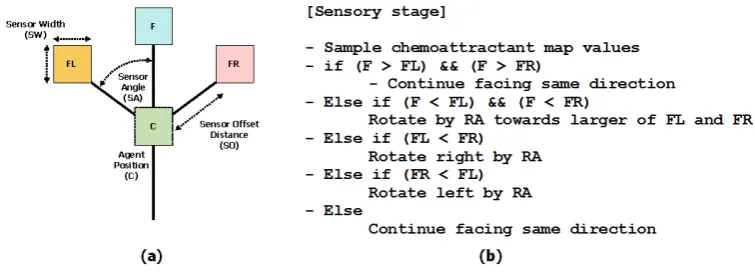
For the computational modelling of slime mould compressibility we employ the multi-agent model introduced in [15]. An overview of the approach can be found in [16]. In the multi-agent approach the Physarum plasmodium is approximated by a population of simple mobile particles. Each particle corresponds to a hy-pothetical unit of gel/sol structure within the Physarum plasmodium. Particles sense and deposit a generic chemo-attractant substance within a 2D diffusive lattice. The current pattern of the particle population represents both the structure and flux within the plasmodium. Particles orient themselves towards the locally strongest source of attractant, as sampled by its three offset sen-sors. Each particle attempts a movement forwards in its current orientation and deposits attractant at the new site if the movement is successful. The offset sensors effect an indirect and local coupling of the particles and the movement of a particle attracts nearby particles, forming an auto-catalytic process where self-organised networks spontaneously form and minimise in shape. The model is notable for its quasi-physical emergent behaviours including network adapta-tion and minimisaadapta-tion. The architecture of a single particle is given in Fig. 1. Particle parameters Sensor Angle (SA), Rotation Angle (RA) generate a com-plex range of Turing-type patterns [14] and the Sensor Offset distance (SO) acts as a pattern scaling parameter.

Figure 1: Single agent particle. (a) agent morphology showing position ‘C’ and three forward biased sensors ‘FL’, ‘F’ and ‘FR’, (b) agent sensory algorithm governing orientation.

by multiplying by 0.9 per scheduler step.

Growth and shrinkage of the particle population is implemented as follows. If there are 1 to 20 particles in a 9×9 neighbourhood of a particle, and the particle has moved forwards successfully, the particle attempts to spawn a new particle if there is a space available at a randomly selected empty location in the immediate 3×3 neighbourhood surrounding the particle. The dependence on successful movement ensures that population growth occurs only in response to the presence of nutrient stimuli. When all nutrients have been discovered, their projection of attractants is suppressed, causing the population to automatically shrink in size using the following test. If there are 0 to 24 particles in a 5×5 neighbourhood of a particle the particle survives, otherwise it is deleted. Dele-tion of a particle leaves a vacant space at this locaDele-tion which is filled by nearby particles, causing the collective to shrink slightly. As the process continues the population shrinks and adapts its morphology to the configuration of stimuli. The frequency of testing for particle division and particle removal was every 3 scheduler steps.

2.3

Expressing compressibility

We express compressibility s(t) of a system as a ratio of the size f(mt) of the compressed image mtof the system to the compressed size f(m1) of the start image m1 taken at the beginning, t = 1 of experiment: s(t) = f(mt)/f(m1). Typical compression utilities, like UNIX utility GZIP work well to represent the measures of compressibility [18, 19, 9].

3

Results

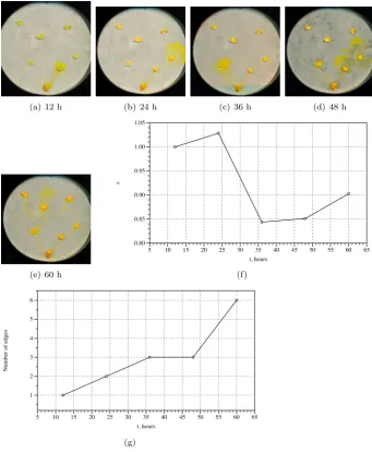
(a) 12 h (b) 24 h

(c) 36 h (d) 48 h (e) 60 h

s

0.96 0.98 1.00 1.02 1.04 1.06 1.08 1.10

t, hours

5 10 15 20 25 30 35 40 45 50 55 60 65

(f)

Figure 2: Physarum approximate Voronoi diagram [2]. (a–e) Photographs of the experimental setup taken in 12 h intervals. See details of setup in [2]. (f) Dynamic of compressibilitys(t).

in complexity. The path in a maze problem shows how compressibility reflects formation of scouting branches.

3.1

Voronoi diagram

of P, a region corresponding to a unique point pcontains all those points of the plane which are closer topthan to any other node of P. A unique region

vor(p) = {z ∈ R2 _{: d(p, z) < d(p, m)∀m ∈ R}2_{, m 6= z} assigned to point} p is called a Voronoi cell of the pointp. The boundary of the Voronoi cell of pointpis built of segments of bisectors separating pairs of geographically closest points of the given planar setP. A union of all boundaries of the Voronoi cells determines the planar Voronoi diagram: V D(P) =∪p∈P∂vor(p) [13].

Planar data pointsPare represented by oat flakes colonised by Physarum. Physarum approximates the Voronoi diagram on a nutrient agar. Therefore it propagates as omnidirectional disc from each site of its inoculation (Fig. 2a). When two waves, originated from geographically neighbouring sites of inocu-lation, meet with each other they stop propagation (Fig. 2b). Thus loci of substrate unoccupied by Physarum represent edges of the Voronoi diagram. By calculations(t) of the experimental images (Fig. 2f) we found that sizes of im-ages grow initially. They reach their maximum values by 36 h of experiment, when majority of the bisectors are formed (Fig. 2c). Then the sizes of im-ages start declining (Fig. 2d). They reach their minimum size by 60 h when Physarum halts it propagation (Fig. 2e).

Using the model plasmodium we repeated the procedure described in [17] where oat flakes representing planar data points were inoculated with particles (Fig. 3, white regions) and nutrient-rich background substrate was represented by grey colour. The model population propagates outwards in an omnidirec-tional disc pattern (Fig. 3b-c), attracted by the stimulus from the background substrate. The Voronoi bisectors in the model population are represented by dense regions of particle occupancy (Fig. 3e). The graph in Fig. 3g of s(t) indicates that the filesize increases as the individual inoculation sites grow. As the Voronoi bisectors begin to emerge (Fig. 3d), the curve begins to flatten out and the filesize then reduces as the bisectors form completely and ultimately merge. This suggests that the plateau in growth of the population (and file-size) may indicate the time when the computation of the Voronoi diagram is approximated.

3.2

Spanning trees

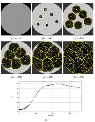
The Euclidean minimum spanning tree [21] is a connected acyclic graph which has minimum possible sum of edges’ lengths. Physarum computes spanning tree on a non-nutrient substrate (Fig. 4). Planar points of the data set are represented by virgin oat flakes, not colonised by the slime mould. One of the data point is assigned to be a root, it is represented by oat flake colonised by the Physarum. In 12 h after inoculation the slime mould propagates along gradients of chemo-atractants towards virgin oat flake closest to the site of Physarum inoculation (Fig. 4a). Then the slime mould continues colonising oat flakes until all data points are spanned by protoplasmic tubes (Fig. 4b–e). Formation of densely branching active growing zones is reflected in increase of image size (Fig. 4b). The more oat flakes (data points) become spanned the less active growing zone emerge and thus sizes of compressed Physarum pattern decrease (Fig. 4f). Complexity of graph constructed increases almost linearly (Fig. 4f).

(a) t=10 (b) t=60 (c) t=120

(d) t=150 (e) t=210 (f) t=330

s

0 2 4 6 8 10 12

t, hours

0 100 200 300

(g)

(a) 12 h (b) 24 h (c) 36 h (d) 48 h

(e) 60 h

s

0.80 0.85 0.90 0.95 1.00 1.05

t, hours

5 10 15 20 25 30 35 40 45 50 55 60 65

(f)

N

um

be

r of e

dge

s

1 2 3 4 5 6

t, hours

5 10 15 20 25 30 35 40 45 50 55 60 65

(g)

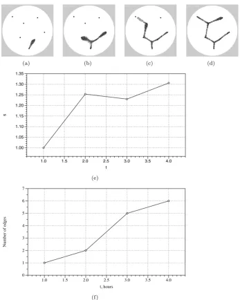
(a) (b) (c) (d)

s

1.00 1.05 1.10 1.15 1.20 1.25 1.30 1.35

t

1.0 1.5 2.0 2.5 3.0 3.5 4.0

(e)

N

um

be

r of e

dge

s

0 1 2 3 4 5 6 7

t, hours

1.0 1.5 2.0 2.5 3.0 3.5 4.0

(f)

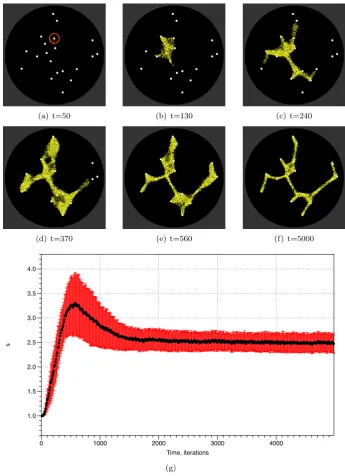
of the graph. We also investigated the behaviour of the model in response to more complex datasets. We randomly generated 20 points (corresponding to oat flakes) on a 300×300 lattice and inoculated the model plasmodium on a randomly chosen point (Fig. 6a, circled). We recorded images of the configuration of the model every ten steps and ran each experiment for 5,000 steps. A typical pattern of growth and adaptation is shown in Fig. 6a-f. From its inoculation site the model plasmodium extended pseudopodium-like processes to migrate towards and engulf each nutrient source. When all the nutrients were covered the resultant reduction in stimuli caused the shape of the population to adapt and minimise to conform to the shape of the points. We recorded the filesizes over ten experiments and the plot of dynamics of averages(t) is shown in Fig. 6g (thick line is aerage, standard deviation error bars indicated by shaded regions). The plot shows an increase insuntil all nodes are discovered (typically t=500-600 steps). The adaptation phase is indicated by the downward slope (600-1000 steps) of s and the stable configuration then continues and is represented by the relatively stable svalue.

To what extent does the increase in population size affect changing com-pressibility? It is possible to argue that the increase and decrease in file size (and subsequent decrease and increase in compressibility) is merely due to the increase and decrease in population and that the re-distribution of the plas-modium (real and virtual) does not affect compressibility. Using the model it is possible to have a ‘fixed size’ plasmodium which does not differ in the number of its components throughout an experimental run. Therefore any changes in com-pressibility must arise as a consequence of the self-organised network formation and adaptation. An example can be shown in Fig.7 in which we use a fixed pop-ulation size of 4000 particles inoculated within a circular arena on a 200×200 lattice containing 50 nutrient sources. The population is initialised at random locations within the arena. Particle sensor parameters were SA 45 and RA 45 and SO was 7. Because growth and shrinkage of the population was disabled we reduced the concentration of the stimuli to 2.5 units per scheduler step and increased particle deposition to 5 units per step. This adjustment is necessary to prevent defects forming in the material from very high concentration stimuli. Fig. 7 shows significant events in the evolution of the fixed sized model plasmodium. Initially there is no network (Fig. 7a) but a network composed of particles connecting the nutrient sources spontaneously forms (Fig. 7). This network undergoes minimisation over time, reducing the number of edges and cycles. The associated graph does not show the initial increase in s(t) as the population size is fixed. Instead s(t) decreases rapidly as the network forms and minimises. The evolution of s(t) then stabilises over time, falling only at significant events in the network evolution (for example, when some remaining cycles are minimised, Fig. 7e,f,g and h). This result demonstrates that the changes in compressibility cannot be due only to changes in population size but also represent the inherent ordering of the networks over time.

3.3

Maze

(a) t=50 (b) t=130 (c) t=240

(d) t=370 (e) t=560 (f) t=5000

s

1.0 1.5 2.0 2.5 3.0 3.5 4.0

Time, iterations

0 1000 2000 3000 4000

(g)

(a) t=1 (b) t=30 (c) t=400 (d) t=1000

(e) t=5000 (f) t=20000 (g) t=27650 (h) t=35000 (i)

Figure 7: Dynamics ofsduring formation and adaptation of proximity graph in the model plasmodium. (a) model plasmodium of 4000 particles is inoculated at random sites within a 200×200 lattice of 50 data points, (b-h) Self-organised network formation and adaptation of model plasmodium as it adapts its shape to locations of attractants, (i) plot of dynamics of s over experiment, initial rapid fall is followed by a long stable periods, punctuated only by removal of cycles within the network.

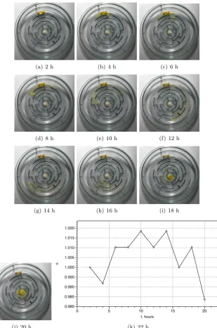
(Fig. 8bcd). By the time diffusing chemo-attractants reached distant channels one of the active zone already became dominant and suppressed another ac-tive zone (Fig. 8efg). In example shown acac-tive zone travelling contra-clockwise dominated and ’extinguished’ active zone propagating clockwise. The dominat-ing active zone then followed gradient of chemo-attractants inside the maze, navigated along intersections of the maze’s channels and solved the maze by entering its central chamber (Fig. 8hij). Spatio-temporal dynamic of space ex-ploration by Physarum is well reflected in the dynamics of compressibility shown in Fig. 8k. Thus formation of branching active zones, or scouting branches at 10 h and 12 h of experiment, is reflected by peaks of compressibility s. When competition between active zones exploring various pathways ends in favour of one of the active growing zone, losers retract. These events lead to drops in compressibility, as e.g. in 12 h and 16 h of experimenting. When the Physarum finds the central chamber all scouting branches retract, or become abandoned, and the compressibility drops to its lowest level, indicating that the solution is found.

3.4

Transport networks

corre-(a) 2 h (b) 4 h (c) 6 h

(d) 8 h (e) 10 h (f) 12 h

(g) 14 h (h) 16 h (i) 18 h

(j) 20 h

s

0.980 0.985 0.990 0.995 1.000 1.005 1.010 1.015 1.020

t. hours

0 5 10 15 20

(k) 22 h

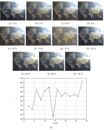
(a) 2 h (b) 4 h (c) 6 h (d) 8 h

(e) 10 h (f) 12 h (g) 14 h (h) 16 h

(i) 18 h (j) 20 h (k) 22 h

s

540 550 560 570 580 590 600 610 620 630

t, hours

0 5 10 15 20 25 30

(l)

sponds to increases activity of the slime mould: it propagates simultaneously from China to Japan and from India to Pakistan (Fig. 9c). At 10 h we can ob-serve an scouting active zone sprouting through China to Russia (Fig. 9e); the active zone does not succeed and detracts back by 12 h. Another peak of image size (decrease in compressibility) is observed at 12 h (Fig. 9l). This reflects developing of several pseudopodia spreading into Africa (Fig. 9f). The coloni-sation of Africa completes by 16 h (Fig. 9gh) which is manifested in substantial increase of compressibility, decrease of the image size (Fig. 9l). At 16 h also London is colonised and Physarum propagates into the North Europe (Fig. 9h) and we see corresponding peak in the image size: increased activity decreases compressibility. Another attempt, this time successful, to colonise Russian terri-tory is made at 18 h (Fig. 9i). By 20 h the slime mould reaches Moscow (Fig. 9j) and recolonizes London again by 22 h (Fig. 9j). These activities do not change compressibility substantially because major part of Eurasia is already colonised by that time.

4

Discussion

Unconventional computers made of physical, chemical and living substrates rarely halt. Even when they find a solution to the given problem, they express their finding via morphological, chemical or electrical changes but then continue their ’daily business’ as if nothing happened. Turing machine halts. Physarum machines never halt. We propose to use dynamics of compressibility of a sys-tem’s spatial configurations to detect when the system completed computation. Compressibility of a system is inversely proportional to morphological diversity — a number of distinct local sub-configurations — of the system. When the system searchers for a solution of the problem it explores the space but also explores itself thus generating a vast number of different spatial sub-states. The patterns of the system in such states are difficult to compress. Compressibility of a system decreases when the system is looking for a solution. When the solu-tion space explorasolu-tion is abandoned the system returns to its state of minimal energy. Compressibility of such system increases. Thus by observing dynamics of the system’s compressibility we can detect when the compressibility stabilised or increased to it maximum. We can conjecture that in that moment the system produces the solution to the problem.

References

[1] Mateo Aboy, Roberto Hornero, Daniel Ab´asolo, and Daniel ´Alvarez. In-terpretation of the Lempel-Ziv complexity measure in the context of biomedical signal analysis. Biomedical Engineering, IEEE Transactions on, 53(11):2282–2288, 2006.

[2] Andrew Adamatzky. Physarum machines: encapsulating reaction–diffusion to compute spanning tree. Naturwissenschaften, 94(12):975–980, 2007. [3] Andrew Adamatzky. Physarum machines: computers from slime mould,

volume 74. World Scientific, 2010.

[4] Andrew Adamatzky. On diversity of configurations generated by excitable cellular automata with dynamical excitation intervals. International Jour-nal of Modern Physics C, 23(12), 2012.

[5] Andrew Adamatzky. Slime mold solves maze in one pass, assisted by gradient of chemo-attractants. NanoBioscience, IEEE Transactions on, 11(2):131–134, 2012.

[6] Andrew Adamatzky. The world’s colonization and trade routes formation as imitated by slime mould. International Journal of Bifurcation and Chaos, 22(08), 2012.

[7] Andrew Adamatzky and Leon O Chua. Phenomenology of retained re-fractoriness: On semi-memristive discrete media. International Journal of Bifurcation and Chaos, 22(11), 2012.

[8] Andrew Adamatzky and Genaro J Martinez. On generative morphological diversity of elementary cellular automata. Kybernetes, 39(1):72–82, 2010. [9] Hussein Al-Bahadili and Ahmad Rababa’a. A bit-level text compression

scheme based on the hcdc algorithm. International Journal of Computers & Applications, 32(3):355, 2010.

[10] Jos´e M Amig´o, Janusz Szczepa´nski, Elek Wajnryb, and Maria V Sanchez-Vives. Estimating the entropy rate of spike trains via Lempel-Ziv complex-ity. Neural Computation, 16(4):717–736, 2004.

[11] Joydeep Bhattacharya et al. Complexity analysis of spontaneous EEG.

Acta neurobiologiae experimentalis, 60(4):495–502, 2000.

[12] David P Feldman and Jim Crutchfield. A survey of complexity measures.

Santa Fe Institute, USA, 11, 1998.

[13] P Preparata Franco, Michael Ian Shamos, and M Ian. Computational Ge-ometry, an introduction. Springer-Verlag, New York, 1985.

[14] Jeff Jones. Characteristics of pattern formation and evolution in approx-imations ofPhysarum transport networks. Artificial Life, 16(2):127–153, 2010.

[16] Jeff Jones.From Pattern Formation to Material Computation: Multi-agent Modelling of Physarum polycephalum. Springer, in-press 2015.

[17] Jeff Jones and Andrew Adamatzky. Slime mould inspired generalised Voronoi diagrams with repulsive fields. Int. J. Bifurcation and Chaos, In-Press, 2013.

[18] Pavel G Khalatur, Viktor V Novikov, and Alexei R Khokhlov. Conformation-dependent evolution of copolymer sequences. Physical Re-view E, 67(5):051901, 2003.

[19] Toshiko Matsumoto, Kunihiko Sadakane, Hiroshi Imai, and Takumi Okazaki. Can general-purpose compression schemes really compress DNA sequences. Currents in Computational Molecular Biology, pages 76–77, 2000.

[20] Toshiyuki Nakagaki. Smart behavior of true slime mold in a labyrinth.

Research in Microbiology, 152(9):767–770, 2001.

[21] Jaroslav Neˇsetˇril, Eva Milkov´a, and Helena Neˇsetˇrilov´a. Otakar Boruvka on minimum spanning tree problem translation of both the 1926 papers, comments, history. Discrete Mathematics, 233(1):3–36, 2001.

[22] Shigeru Ninagawa. Solving the parity problem with Rule 60 in array size of the power of two. arXiv preprint arXiv:1307.3888, 2013.

[23] Shigeru Ninagawa and Andrew Adamatzky. Classifying elementary cellular automata using compressibility, diversity and sensitivity measures. Inter-national Journal of Modern Physics C, 25(03), 2014.

[24] Shingeru Ninagawa and Genaro J Martinez. Compression-based analysis of cyclic tag system emulated by Rule 110. J. Cellular Automata, 9(1):23–35, 2014.

[25] Yuri L. Orlov and Vladimir N Potapov. Complexity: an internet resource for analysis of DNA sequence complexity. Nucleic acids research, 32(suppl 2):W628–W633, 2004.

[26] Markus Redeker, Andrew Adamatzky, and Genaro J Mart´ınez. Expres-siveness of elementary cellular automata. International Journal of Modern Physics C, 24(03), 2013.

[27] Steven L Stephenson, Henry Stempen, and Ian Hall. Myxomycetes: a handbook of slime molds. Timber Press Portland, Oregon, 1994.