Optimizing interpreters by tuning opcode orderings on virtual machines for modern architectures

Optimizing Interpreters by Tuning Opcode Orderings

on Virtual Machines for Modern Architectures

Or: How I Learned to Stop Worrying and Love Hill Climbing

Jason McCandless

David Gregg

Trinity College Dublin Lero@TCD

{mccandjm,dgregg}@cs.tcd.ie

Abstract

Virtual machines (VMs) are commonly used to implement pro-gramming languages such as Java, Python and Lua. VMs are typ-ically implemented using an interpreter, a JIT compiler, or some combination of the two. A long-standing question in the design of VM interpreters is whether it is worthwhile to reorder the cases in the main interpreter loop to improve code locality. We investigate this phenomenon using an iterative, feedback-directed approach. We show that the ordering of the cases in the interpreter loop has a significant impact on performance on recent processors. Using hardware performance counters, we demonstrate that the perfor-mance improvement is primarily the result of indirect branch pre-diction, not instruction cache locality. We propose a number of strategies to achieve better orderings, and evaluate these strate-gies in the Python and Lua virtual machine interpreters. We show speedups of up to 40%.

Categories and Subject Descriptors D.3.4 [Software]: Program-ming Languages — Processors — Interpreters

General Terms Languages, Performance, Experimentation

Keywords Virtual machines, Lua, Python, Locality, Branch pre-diction

1.

Introduction

Virtual machine interpreters are widely used to implement pro-gramming languages such as Java, Lua and Python.

Interpreters are much slower than the native code produced by just-in-time compilers (even the fastest interpreters are around 5-10 times slower), but they have several advantages that can make them attractive. If an interpreter is written in a high-level language such as C, it can be made portable, and can simply be recompiled for a new target architecture. In contrast, retargetting a just-in-time (JIT) compiler can require a lot of effort. Interpreters also require little

∗_{Supported by the Irish Research Council for Science, Engineering &}

Technology.

[Copyright notice will appear here once ’preprint’ option is removed.]

memory: the interpreter itself is typically much smaller than a JIT compiler [19], and the interpreted bytecode is usually a fraction of the size of the corresponding executable native code. For this reason, interpreters are commonly found in embedded systems, or systems such as games, where the memory budget is carefully divided among the components of the system. Furthermore, if the application consists of a lot of code, interpreting rarely-executed code can actually befasterthan JIT compilation. This is the basis of many hybrid interpreter/JIT systems that interpret the bulk of the code, and JIT compile the hotspots. A further advantage is that the interpreter can collect information about the program as it runs, which can be useful for JIT compilation. Interpreters are also dramatically simpler than compilers; they are easy to construct, and easy to debug. Finally, it is easy to provide tools such as debuggers and profilers when using an interpreter because it is easy to insert additional code into an interpreter loop. Providing such tools for native code is much more complex. These advantages make interpreters common among language implementations.

Language implementations based on virtual machines (VMs) typically compile high-level source code into an array of opcodes (bytecodes). They then use an interpreter to execute the array of opcodes. Often this interpreter is written in C and uses a large

switchstatement to select the appropriate code to execute for the current opcode. The code implementations (switch cases) of these opcodes are usually laid out in an ad-hoc manner1. The most common ordering in the source code of VMs we have seen is the numeric order of the corresponding opcodes.

A reasonable question to ask is whether the order of the cases in the interpreter loop can have a significant impact on performance. For example, if the commonly executed cases are kept together, then it may improve code locality. Sun Microsystem’s K Virtual Machine for embedded Java [20] does exactly this, which suggests that there may be real benefits from code locality. There may also be less obvious benefits. For example, arbitrary changes in the order of code may change the relative positions of conditional branches, which may result in fewer collisions in the branch predictors. Fi-nally, arbitrary reorderings of code can have almost arbitrary ef-fects on performance. For example, even code that is never exe-cuted can have an impact on performance if it is fetched into the processor pipeline. The less obvious benefits are much more diffi-cult to model than locality effects, and it is thus diffidiffi-cult to design code optimization strategies that take advantage of them. However, it is valuable to discover the extent to which these arbitrary out-comes can improve performance.

1_{Since compiler optimizations often move code around, this might be}

We are not the first to investigate the question of ordering the cases within the interpreter loop to improve locality. Brunthaler [5], who refers to this problem as interpreter instruction scheduling2_,

provides an algorithm to reorder cases to improve locality, and reports speedups for a modified Python interpreter.

In this paper we address the case ordering question for VM interpreters, but take a different approach. In addition to improving locality we also want to investigate other effects of case reordering. We therefore take a feedback-directed iterative approach to finding good case orderings. This allows us to capture other speedups beyond those resulting in improved locality, and investigate their causes. This paper makes a number of contributions:

•We evaluate Brunthaler’s [5] graph selection approach in our experimental framework and present results.

•We propose an iterative solution based on the Monte Carlo method, showing it to be a reasonable search method for this problem.

•We evaluate two alternatives to this method, based on hill climbing and simulated annealing.

•We apply our methods to the Python 2.6, Python 3.2, and Lua 5.1 interpreters. We measure the difference the effect has between switch and token-threaded interpreters, and present results for the Intel Core and Nehalem architectures.

•Using hardware performance counters, we demonstrate that in our experiments performance improvements from code reorder-ing are not primarily the result of improved locality.

•We show that on recent processors the performance impact of case reordering is primarily the result of its effect on indirect branch prediction.

2.

Background

Some of the computer architecture subsystems that typically influ-ence program performance are instruction cache, data cache, and branch prediction. Interpreters suffer from these influences also. An interpreter does not usually stall waiting for data, so we focus our attention on instruction cache and branch prediction misses.

Instruction caches rely on the property that program flow is highly predictable, and therefore instruction memory access is pre-dictable (it has good spatial and temporal locality). If a programmer wants to improve the cache behavior, she should generate the small-est code possible and additionally, improve prefetching through code layout, or use explicit prefetching.

CPU pipelines have grown over time, and modern processors have highly sophisticated branch predictors that attempt to avoid branch misprediction and a flush of the pipeline. Effective branch predictors are so important for performance that they are a compet-itive edge for CPU manufacturers, so their specific behavior is not publicly documented. There have been attempts to reverse engineer the exact details of branch predictors [1].

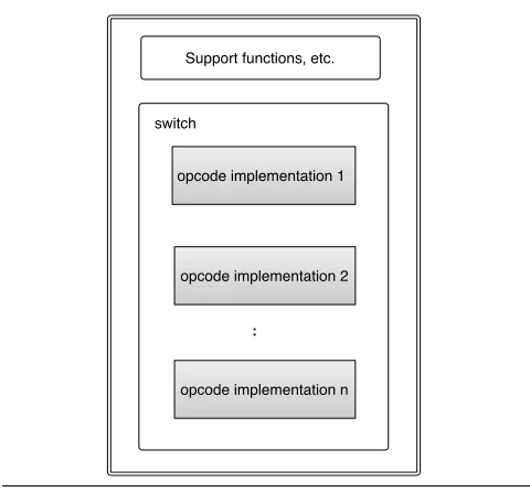
An interpreter is frequently written in C, with code fragments that implement the instruction set of the virtual machine. Opcode ordering is the arrangement of the implementations of opcodes in memory. Figure 2 shows the typical layout of an interpreter core. Here we presume it is a switch interpreter; however, direct and indirect threaded interpreters will be structured in a similar fashion. Lua 5.1 is a register virtual machine with a switch-based inter-preter and has 38 opcodes. Python 2.6 is a stack virtual machine with a switch-based interpreter and has 112 opcodes. Python 3.2 is token-threaded [3] when compiled with a compiler that supports

la-2_{We refer to the concept as ordering, as scheduling implies a temporality}

property, which is not the case here.

Support functions, etc.

switch

opcode implementation 1

opcode implementation 2

opcode implementation n

..

Figure 1. Typical interpreter structure.

bels as values (computed goto), otherwise switch-based. It has 100 opcodes.

3.

Best-first

To find a good ordering, perhaps the most ‘obvious’ choice would be to arrange the opcode implementations such that the most fre-quent are clustered together at the top of the interpreter dispatch loop. Indeed it appears that this is a common practice amongst in-terpreter designers: we seeLOAD_FASTappear at the top of the Python dispatch loop, andOP_MOVEappear at the top of the Lua dispatch loop.

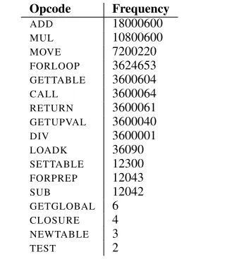
As a concrete example, Table 1 shows the frequencies of various opcodes for the spectral norm benchmark. The most frequent op-code,ADDwould be the first opcode implementation in the memory address space, and similarly for the following opcodes.

We implement ordering based on frequency for the Lua and Python interpreters by aggregating opcodes from profiles we collect by running the various benchmarks in our set. We place the most frequently executed ones at the top of theswitch.

An issue with the Python implementation is the use of ‘fall through’ semantics for the overlapping implementations of some opcodes. For instance the implementation of thePRINT_ITEM_TO opcode (which prints the item second from the top of stack) shown in Figure 2 has only one extra statement compared to the PRINT_ITEM opcode, so the implementations are overlapped to save code memory. This is a complication, since our opcode traces will have two different opcodes. We do not want to consider dupli-cate implementations3. We solve this by mapping these extended opcodes to their parent opcode — we are only considering opcode implementations, not opcodes.

Our traces include the start-up functions of the Python inter-preter. That is, 70,394 opcodes in Python 2.6, and 823060 opcodes in Python 3.2. A slight caveat is that we convert the parallel

bench-3_{A potential approach might be to split the opcodes, however we have}

Opcode Frequency

ADD 18000600

MUL 10800600

MOVE 7200220

FORLOOP 3624653 GETTABLE 3600604

CALL 3600064

RETURN 3600061

GETUPVAL 3600040

DIV 3600001

LOADK 36090

SETTABLE 12300

FORPREP 12043

SUB 12042

GETGLOBAL 6

CLOSURE 4

NEWTABLE 3

TEST 2

Table 1. Opcode frequencies for the Lua spectral norm bench-mark, showing a possible ordering from most frequent to least fre-quent.

case PRINT_ITEM_TO: w = stream = POP();

/* fall through to PRINT_ITEM */

case PRINT_ITEM: v = POP(); ...

break;

Figure 2. Problem of joined opcode implementations in Python. The two opcodes implement almost identical functionality, so a ‘fall though’ between cases is used to avoid code duplication.

marks (mandelbrot & binary-trees) to sequential equivalents in or-der to get a coherent trace4_.

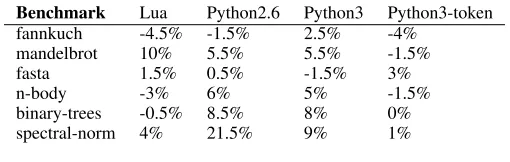
Tables 2 and 3 show the speedups from best-first ordering on the Core 2 and Nehalem machines respectively (rounded to the near-est 0.5%). Our experimental methodology is described in Section 8. We observe some speedups, but also some slowdowns. These results suggest that best-first is not a good heuristic for ordering opcode implementations.

4.

Graph Selection

Brunthaler [5] presents the problem of finding a good ordering as a graph problem, where the vertices represent opcodes and the edges represent the frequency of transitions between opcodes (collected from a profile). This graph is a weighted directed graph that is weakly connected. We wish to find a tour that visits each vertex once, and maximises the cost function. This problem is similar to the asymmetric travelling salesman problem, where the triangle inequality does not hold. However the graph is incomplete, so it also resembles the Hamiltonian path problem. This is not exactly right either though, since a tour is permitted to include edges that do not exist in the graph. These edges may be added because it is legal to place opcode implementations adjacent to each other even if they do not form a pair in the profile used to construct the graph.

4_{With our mandelbrot benchmark for Python 3, which uses a concurrent}

worker-writer model, we could not remove the concurrency beyond a mini-mum of two processes.

Benchmark Lua Python2.6 Python3 Python3-token

fannkuch -3% -1% 5% -4%

mandelbrot 10% 2% 6.5% 2.5%

fasta 4.5% -1.5% -1% 2.5%

n-body -0.5% 1.5% 6.5% 0%

binary-trees -7.5% 10.5% 6.5% 0% spectral-norm 5.2% 13.5% 5.5% -4%

Table 2. Best-first speedups on Core 2.

Benchmark Lua Python2.6 Python3 Python3-token

fannkuch 8% 13% -2.5% -0.5%

mandelbrot 32.5% 17% 6.5% -0.5%

fasta 10.5% 8.5% 0% 1%

n-body 0% 10% 4.5% 2.5%

binary-trees -1% 3.5% 1.5% 0%

spectral-norm 5% 17% 0% 0.5%

Table 3. Best-first speedups on Nehalem.

The only guaranteed tour in the graph (without adding extra edges) is the tour formed by the sequence of opcodes from the profile.

Algorithm 1Brunthaler’s graph selection algorithm

1: schedule← ∅ 2: open←sorted(graph)

3: whileopen6=∅do 4: n←largest(open)

5: whilendo

6: schedule←schedule∪{n}

7: reachable←sorted(n.destinations)\schedule

8: n←false

9: ifreachable6=∅then 10: n←largest(reachable)

11: open←sorted(reachable∪open)

12: end if

13: end while

14: end while 15: return schedule

In Algorithm 1, we outline the graph selection algorithm de-scribed by Brunthaler.Scheduleandopenare ordered sets. The algorithm is similar to the classical nearest neighbour (greedy) al-gorithm [2], with some differences:

• Revisiting a vertex is permitted.

• If we reach a ‘dead-end’ (recall that the graph is not complete) then the next node is fetched from theopenset.

• The final difference is the open set updating:

open←sorted(reachable∪open)

Items reachable from the present node are added to theopen list. These items will have higher precedence, because items initially put in the open list are sorted, but are placed in with weight 0 (the ordering of the original nodes is not affected, since a stable sort is used).

As an example, applying the algorithm to the profile graph shown in Figure 3 yields the ordering: {FORLOOP,GETGLOBAL, MOVE,CALL,RETURN,FORPREP,LOADK}.

loadk

forprep

forloop

return getglob

move call

1

1

1

3 3

3 3

Figure 3. Opcode profile graph for the Lua program: ‘for i = 1,3 do print(i) end’.

applying the algorithm to the traces of those kernels, we apply the algorithm to traces of whole programs. This should not have detri-mental effects, as the algorithm selects for frequency, so infrequent opcodes should get relegated in any case.

Brunthaler provides Python source and we base our implemen-tation on this [5]. We evaluate his graph technique for the Lua, Python 2.6 and Python 3.2 interpreters on the Core 2 and Nehalem machines. The results we found are shown in Tables 4 and 5.

These results show the speedups (and slowdowns) when an or-dering found from the trace of a benchmark is evaluated on that benchmark. Better speedups are possible when we do not restrict what benchmark an ordering was tuned on, and instead try all the possible orderings generated from traces of the different bench-marks. We do not present those numbers here, as the algorithm is meant to find good orderings for the trace it is presented with.

To improve upon these results, a better algorithm than the greedy algorithm could be used to minimize the global distance of a tour (an optimal solution might be possible inO(2n)). However, we do not explore this — since an ordering tuned from a particular benchmark is not always the best ordering for that benchmark, it must follow that the graph technique is modelling the wrong thing. We instead now look at orderings generated stochastically.

5.

Monte Carlo Generation

In the previous two sections we looked at opcode frequency based methods to layout opcodes in memory. The results we found were unsatisfactory. We now investigate a more general, combinatorial technique. We want to find the opcode ordering that has the low-est execution time (our cost function). The combinatorial search space of all possible opcode orderings is every permutation, which isO(n!)complexity for a brute force approach. Since most inter-preters have more than thirty opcodes, this search space will be upwards of1032(For Lua, which has a relatively low number of opcodes (38), there are over1044permutations). Without any in-dication of an optimal algorithm, we investigate stochastic search methods.

Monte carlo methods are used to model phenomena with sig-nificant uncertainty in inputs. With Monte Carlo generation of or-derings, we randomly (from an underlying uniform distribution) permute the opcodes, compile the interpreter and evaluate it on a set of benchmarks, recording the best time observed so far.

The combinatorial complexity of all possible opcode orderings is similar to that of finding the shortest tour in the travelling sales-man problem. Hence we can borrow the theorem that to stochasti-cally achieve a result that is within1 +1_c of the optimal solution

Benchmark Lua Python2.6 Python3 Python3-token

fannkuch -4.5% -1.5% 2.5% -4%

mandelbrot 10% 5.5% 5.5% -1.5%

fasta 1.5% 0.5% -1.5% 3%

n-body -3% 6% 5% -1.5%

binary-trees -0.5% 8.5% 8% 0%

spectral-norm 4% 21.5% 9% 1%

Table 4. Graph selection speedups on Core 2.

Benchmark Lua Python2.6 Python3 Python3-token

fannkuch 7.5% 8.5% -7% -0.5%

mandelbrot 8.5% 17% -0.5% -4%

fasta 9% 7.5% 0.5% 0.5%

n-body -3.5% 9% 1.5% 1.5%

binary-trees 2.5% 6% -1.5% -1%

spectral-norm 2% 9% 4.5% -6%

Table 5. Graph selection speedups on Nehalem.

1.10 1.15 1.20 1.25 1.30 1.35 Execution time

0 10 20 30 40 50 60

Coun

t

Figure 4. Histogram showing the frequencies of different ordering execution times found by Monte Carlo sampling for the mandelbrot benchmark on Python 3 (switch).

0 500 1000 1500 2000 2500 3000

Number of iterations 0.68

0.70 0.72 0.74 0.76 0.78 0.80 0.82 0.84

Execution

time

(cost)

for TSP with at least 50% certainty, requires the following com-plexity:O(n2cO(1)_+nlogn)

[11, p. 282]. With this exponential decrease, we rapidly stop seeing improvements. We see this in our experimental observations similarly.

An example of Monte Carlo generation is shown in Figure 4. The figure shows a histogram of the execution times for the various opcodes orderings generated for the mandelbrot benchmark. This example is for the Python 3 switch interpreter on our Core 2 ma-chine. Figure 5 shows the progress of the Monte Carlo method over time for the fannkuch benchmark. This is for the Lua interpreter on our Core 2 machine.

Table 6 summarises the various speedups achieved on the dif-ferent interpreters we measured on the Core 2. These speedups are achieved by running each benchmark with the best possible order-ing found for it. In contrast, Table 7 shows speedups (and an overall average speedup) when just one ordering is used per set of bench-marks. Tables 8 and 9 show the same results, but for our Nehalem machine.

The random permutations for Monte Carlo are generated by the Mersenne twister pseudorandom number generator, which has a period of219937−1[14]. This will work for sequences up to size 2080 (which will have≈219932permutations).

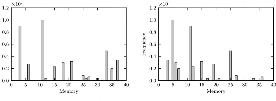
We see respectable speedups from the Monte Carlo approach, but we want a deeper understanding of the cause. Figure 6 shows two memory layouts with opcodes frequencies for the fannkuch benchmark on the Lua interpreter. On the left we see the best ordering found for that benchmark, on the right we see the worst. After inspecting a number of these graphs, we do not see any common visual pattern to account for the performance variations.

6.

Hardware Analysis

We desire a deeper understanding of what is really going on in hardware with the performance variation from different opcode orderings. We will look at cache and branch prediction:

6.1 Cache

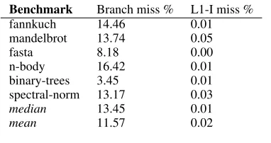
Firstly, we investigate the effect of level 1 instruction cache on the performance of a switch-case interpreter. For our Lua benchmark sample, we do not observe a significant number of instruction cache misses. We evaluate this using Pin and Valgrind with a 32KB 8-way set associative cache (the size of the cache in our Core 2 machine). Additionally, We also record hardware performance counters via PAPI [4]. Finally, we measure the code distance between the be-ginning and end of the switch block by taking the address of labels (this excludes executed code that is in functions outside of the in-terpreter loop; but in Lua, code such as this is often the special case anyway). The total address distance in the Lua interpreter loop is 5953 bytes. This is considerably less than the 32KB level 1 instruc-tion cache on the Intel Core. Addiinstruc-tionally, the full code size of the interpreter is not all going to be needed in the instruction cache — the frequency of opcodes is not distributed in such a uniform man-ner, as the opcode frequency counts of the spectral norm benchmark shown in Table 1 illustrate.

Table 10 shows estimated figures of the percentage of cycles stalled due to L1 misses5. We calculate these from the cycle count of the benchmarks and the L1-I misses as reported by the hardware performance counters. In all cases, the proportion of time lost to L1 instruction cache misses is significantly less than 1%.

5_{We assume a 14 cycle branch penalty (pipeline size) and a 15 cycle L1-I}

miss penalty. Obviously these penalties are highly dynamic in a modern out-of-order superscalar CPU, but our estimates are representative, and show a large difference between cycles stalled due to branch mispredictions and due to cache misses.

Benchmark Lua Python2.6 Python3 Python3-token

fannkuch 5% 18% 17% 5%

mandelbrot 14% 13% 20% 4.5%

fasta 22% 6% 3.5% 4.5%

n-body 5.5% 9% 15% 5%

binary-trees 4% 17% 12% 4%

spectral-norm 7% 39% 22% 1%

Table 6. Monte Carlo generation speedups on Core 2 (individually tuned orderings).

Benchmark Lua Python2.6 Python3 Python3-token

fannkuch 0% 14% 13% 5%

mandelbrot 13% 11.5% 19.5% 4.5%

fasta 18% 3% 2% 4.5%

n-body 3.5% 4.5% 13.5% 5%

binary-trees -1% 14% 9.5% 4%

spectral-norm 4% 38% 18% 1%

geo-mean 6% 14% 12.5% 2.5%

Table 7. Monte Carlo generation speedups on Core 2 (using one pareto optimally tuned ordering).

Benchmark Lua Python2.6 Python3 Python3-token

fannkuch 10% 18% 6% 4%

mandelbrot 40% 20% 13.5% 2.5%

fasta 14% 9.5% 2.5% 1.5%

n-body 3% 18% 9% 2%

binary-trees 4.5% 12.5% 6.5% 3%

spectral-norm 23% 28% 11.5% 2%

Table 8. Monte Carlo generation speedups on Nehalem (individu-ally tuned orderings).

Benchmark Lua Python2.6 Python3 Python3-token

fannkuch 7.5% 16% 1.5% 2.5%

mandelbrot 35% 17% 10% 1%

fasta 12.5% 8.5% -1% 0.5%

n-body -2% 12.5% 6% 0%

binary-trees 1.3% 10.5% 4% 2%

spectral-norm 15% 19.5 10.5% 1%

geo-mean 11.5% 14% 5% 1%

Table 9. Monte Carlo generation speedups on Nehalem (using one pareto optimally tuned ordering).

Benchmark Branch miss % L1-I miss %

fannkuch 14.46 0.01

mandelbrot 13.74 0.05

fasta 8.18 0.00

n-body 16.42 0.01

binary-trees 3.45 0.01

spectral-norm 13.17 0.03

median 13.45 0.01

mean 11.57 0.02

0 5 10 15 20 25 30 35 40 Memory

0.0 0.2 0.4 0.6 0.8 1.0 1.2

F

requency

×107

(a) Opcode memory layout for best ordering found via Monte Carlo.

0 5 10 15 20 25 30 35 40

Memory 0.0

0.2 0.4 0.6 0.8 1.0 1.2

F

requency

×107

(b) Opcode memory layout for worst ordering found via Monte Carlo.

Figure 6. Execution frequency of opcode implementation positions in memory. Both figures show frequencies for the fannkuch benchmark on Lua (38 opcodes).

6.2 Branch Prediction

Since instruction cache misses do not appear to be that much of a concern for the interpreter, we turn to investigating the effect of branch prediction.

Table 10 shows estimated figures of the percentages of cycles stalled due to branch mispredictions. We calculate these from the cycle count of the benchmarks and the branch misses as reported by the hardware performance counters. We see that branch mispre-diction is commonplace and significant.

Branch mispredictions can be caused by conditional branch misses. We looked at those for the orderings generated by our Monte Carlo technique, but did not observe a correlation between conditional branch mispredictions and execution time. The alterna-tive cause of branch mispredictions is indirect branch misses.

Figure 7(a) shows execution times and indirect branch mispre-diction rates for various opcode orderings found through the Monte Carlo method (x-axis is sorted by execution time). It is clear from this figure that ordering affects execution speed mainly through in-direct branch misses. Figure 7(b) shows execution times, total indi-rect branch mispredictions and level 1 instruction cache misses for various opcodes orderings found through Monte Carlo. This figure also shows that the instruction cache is not a significant determi-nant of execution speed (the cache axis is not shown, but it is 25 times smaller than the indirect branch axis).

The low token threaded speedups we witnessed from Monte Carlo generation also support the claim that indirect branch pre-diction is the cause of varying execution speed.

An explanation of the effect of opcode ordering on indirect branch misprediction is that the Core microarchitecture includes an indirect branch predictor like the Intel Pentium M [10]. Uzelac and Milenkovic [21] reverse engineered the indirect branch predictor in the Pentium M. Their work shows that the iBTB is indexed by a path information register, which is updated with a shift andXOR on the 6 least significant bits of the indirect branch target address. Moving opcode implementations in an interpreter will change the bits of the target, and this will lead to changes in accuracy in the path information register, and consequentially changes in the accuracy of indirect branch misprediction.

6.3 Branch prediction as a Cost Function

Since we know that the ordering primarily affects execution time through branch mispredictions, we could also have used the branch misprediction hardware counter while searching for a good

order-ing. We tried this, but found that it was not as good as execution speed, and it was unnecessary to use a proxy in any case. This means that indirect branch prediction is not the only issue, even if it is the dominant one.

7.

Feedback-Directed Search

In the previous sections we looked at frequency-based algorithms to find orderings and an initial metaheuristic based on Monte Carlo generation of orderings. We now explore a more guided approach for finding satisficing orderings.

7.1 Simulated Annealing

Once more inspired by the travelling salesman problem, we use simulated annealing as a ‘smarter’ method to generate a good ordering. The solution search space is coherent, so we can traverse it by transitioning to the next candidate solution by modifying the current one. Simulated annealing is an appropriate heuristic search method as it does not get stuck in local maxima. The diameter of the search space is small, which is good for simulated annealing — we can get from one state to any other inn(n−1)/2steps.

Algorithm 2 shows our simulated annealing algorithm. Our initial candidate is simply the default ordering in the interpreter. Figure 8 shows the progress of the simulated annealing algorithm over time on the fannkuch benchmark on Lua. We evaluated the algorithm for Lua on the Core architecture and present our results in Figure 9. We provide results for individually tuned orderings for each benchmark as well as a global pareto optimal ordering6. We do not see improvements over the best Monte Carlo generated orderings.

7.2 Hill Climbing

With simulated annealing, we did not see any results that were better than Monte Carlo. This is likely because we are limited to a small number of iterations (750), due to the high cost of evaluating each ordering, whereas typical simulated annealing systems might run for millions of iterations. We also may not have found the ideal parameters for simulated annealing — the values for k, cooling fraction and steps per temperature. We did observe progress after the algorithm had cooled and was not accepting bad solutions anymore.

6_{We consider an ordering Pareto optimal if it maximizes the geometric}

0 100 200 300 400 500 0.60

0.65 0.70 0.75

Execution

time

5 10 15 20 25 30 35 40 45 50

Indirect

branc

h

miss

rate

(%)

Execution time

Indirect branch miss rate

(a) Execution times vs. indirect branch misprediction rates for different opcode orderings generated by Monte Carlo (sorted by execution time).

0 100 200 300 400 500

0.60 0.65 0.70 0.75 0.80

Execution

time

0.0 0.5 1.0 1.5 2.0 2.5

Indirect

branc

h

misses

executed

×107

Execution time L1-I misses

Indirect branch misses

(b) Execution times vs. indirect branch mispredictions vs. level 1 instruction cache misses (axis not shown) for different opcode orderings generated by Monte Carlo (sorted by execution time).

Figure 7. Lua interpreter executing the fasta benchmark on Core 2. The two figures show data from different orderings.

0 100 200 300 400 500 600 700 800

Number of iterations 0.59

0.60 0.61 0.62 0.63 0.64 0.65 0.66 0.67

Execution

time

(cost)

Figure 8. Progress over time of simulated annealing on Lua fannkuch benchmark on Nehalem.

0 0.2 0.4 0.6 0.8 1 1.2

fannkuch

mandelbrot

fasta

n−body

binary−trees

spectral−norm

nsieve

fibonacci

matrix−mul _{nested−loops}

Speedup

Baseline Pareto Optimal Indvidual Best

Figure 9. Simulated annealing results for the Lua interpreter on Core 2. Pareto optimal refers to one ordering that works best with all benchmarks.

Algorithm 2Simulated annealing algorithm used to traverse the solution space.

1: cooling_fraction←0.8 2: cooling_steps←30 3: steps_per_temp←100 4: k←1

5: temperature←1 6: current_perm← · · ·

7: current_value←evaluate(current_perm)

8: fori= 0tocooling_stepsdo

9: temperature←temperature×cooling_fraction

10: forj= 0tosteps_per_tempdo

11: possible_solution←random_swap(current_perm)

12: cost←evaluate(current_perm)

13: merit←e(current_value−cost)/(k×temperature) 14: ifcost<current_valuethen

15: current_value←cost

16: current_perm←possible_solution

17: else ifmerit> random[0,1]then 18: current_value←cost

19: current_perm←possible_solution

20: end if

21: end for

22: end for

23: return current_perm

We evaluate hill climbing as a search strategy as it is an ap-proach that converges faster than simulated annealing. The simplest form of hill climbing, steepest ascent, would evaluate every neigh-bor, and transition to the best. However, that is not practical for us, as our neighbors are all the possible switches of pairs in the order-ing and there are n₂pairs, which means that even in Lua, with 38 opcodes, we will have 703 neighbors at each step. Because of this, and our high evaluation cost, we evaluate stochastic hill climb-ing. In particular we do first-choice stochastic hill climbing (always picking the first neighbor if it is uphill).

0 50 100 150 200 250 300 350 Number of iterations

0.590 0.595 0.600 0.605 0.610 0.615 0.620 0.625 0.630

Execution

time

(cost)

Figure 10. Progress over time of the first-choice stochastic hill climbing algorithm on Lua fannkuch benchmark on Nehalem.

0 100 200 300 400 500 600 700 800

Number of iterations 0.540

0.545 0.550 0.555 0.560 0.565

Execution

time

(cost)

Figure 11. Progress over time of the first-choice stochastic hill climbing algorithm with error consideration and periodic restarts algorithm on Lua fasta benchmark on Nehalem.

Algorithm 3 First-choice stochastic hill climbing with periodic restarts (and error consideration) algorithm used to traverse solu-tion space.

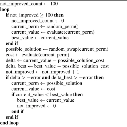
1: not_improved_count←100

2: loop

3: ifnot_improved≥100then 4: not_improved_count←0

5: current_perm←random_perm()

6: current_value←evaluate(current_perm)

7: best_value←current_value

8: end if

9: possible_solution←random_swap(current_perm)

10: cost←evaluate(current_perm)

11: delta←current_value−possible_solution_cost

12: delta_best←best_value−possible_solution_cost

13: not_improved←not_improved+ 1

14: ifdelta>−erroranddelta_best>−errorthen 15: current_perm←possible_solution

16: current_value←cost

17: ifcurrent_value<best_valuethen 18: best_value←current_value

19: not_improved←0

20: end if

21: end if

22: end loop

• Since we are measuring execution time, sampling error is a concern. The hill climbing algorithm is greedy, and will only accept better solutions, but it should also accept equal solutions; in this way it can traverse a plateau and possibly ascend again. However, it is possible to get stuck on a plateau and not make progress if — due to a measurement error while evaluating an ordering — we measure a particularly low execution time. This way, there will be no transitions to neighbors that may have true equal cost, and the algorithm will not make progress. To avoid this scenario, we modify the algorithm to allow transitions to inferior solutions, provided they are within the error range (a figure we find empirically). This change alone would allow gradual descent, so we also keep track of the best value found so far, and refuse to accept transitions to potential solutions that are not within the error range of the best.

• We also perform periodic restarts of the algorithm if no progress is made (an improvement on the best solution is not found) after a fixed number of iterations.

Algorithm 3 shows our modified hill climbing algorithm and Figure 11 shows the progress of this modified algorithm over time for the Lua interpreter running the fasta benchmark. The algorithm restarts if no progress is made in 100 iterations. In this example, it restarts 4 times. We see that is able to make more progress than the naive initial hill climbing algorithm.

Figure 12 shows the results of the algorithm for our benchmark set on our Nehalem machine. The algorithm does not find better individually tuned orderings than the Monte Carlo method, but it does find a better Pareto optimal ordering for the benchmark set, even though we evaluate it using a larger benchmark set than we did for Monte Carlo.

Part of the reason we did not see even larger improvements over Monte Carlo is that algorithms such as hill-climbing and simulated annealing suit a problem best when the cost of incremental evalua-tion is lower than cost of global evaluaevalua-tion. This is not the case here — we must perform a global evaluation on each transition. The cost of evaluating a given ordering is constant, but it is a high constant (approximately 100 seconds per ordering).

8.

Experimental Methodology

8.1 Benchmarks

Our benchmark set is taken from the Computer Language Bench-marks Game [8]. A lack of established benchmark sets for scripting languages makes these suites a common source of benchmarking for scripting language implementations [5, 17].

We use the GCC compiler with the option-fno-reorder-blocksto stop our re-orderings from being negated by basic block reordering performed by the compiler’s software trace cache. We compile both interpreters with maximum optimization (-O3).

When evaluating opcode permutations, we run each bench-marks 15 times, and take the median. While a higher number of runs is obviously more desirable, we found this to be a good trade-off between accuracy and time for our purposes; a larger number would not enable us to evaluate as many candidate solutions. More complex techniques have been proposed by Leather et. al [12] to dynamically determine the number of runs required to eliminate noise in an iterative tuning scenario. Regardless, our results for dif-ferent opcode orderings are fully reproducible.

8.2 Hardware Configuration

We evaluate our techniques on two systems:

0 0.2 0.4 0.6 0.8 1 1.2 1.4 1.6

fannkuch

mandelbrot

fasta

n−body

binary−trees

spectral−norm

nsieve

fibonacci

matrix−mul _{nested−loops}

Speedup

Baseline Pareto Optimal Indvidual Best

Figure 12. First-choice stochastic hill climbing with periodic restarts (and error consideration) results for the Lua interpreter on Nehalem. Pareto optimal refers to one ordering that works best with all benchmarks.

•Intel Core 2 Q6600 (Core Kentsfield) 2.4 GHz CPU with 6 GB memory, running Ubuntu GNU/Linux 10.04 with kernel version 2.6.32-29. GCC version 4.4.3.

8.3 Bytecode Traces

Python provides an internal data structure,dxpairs, that encodes the opcode pair frequencies. However, we opted against using it since it is only practical to access it from a Python program itself, and the bytecodes related to this access code will also get included in the trace. Therefore we simply dumped the opcode numbers from the interpreter as they were executed, and translated these into the appropriate opcode names.

8.4 Compiler Label Alignment

Compilers attempt to make intelligent alignment decisions for code. This is to maximize the amount of code that fits into a cache line, achieving the best hit ratio from the instruction cache (lowest amount of time stalled waiting to fetch code from memory). The GCC compiler can align functions, jumps, labels and loops.

GCC has an option-falign-labels=[n]that allows the program-mer to specify an alignment for labels. We experimented with this option, however we found from assembly inspection that we could only increase the alignment bit count, and not reduce it. We manu-ally removed the alignment pseudo-assembler (.p2align) directives and found a speedup of 1.2% on the fannkuch benchmark with the Lua interpreter. For comparison, disabling reordering for this benchmark led to a 2% speedup. Disabling these two ‘optimiza-tions’ led to a total speedup of 3.3%.

For Python 2 and 3, we did not observe alignment directives between every opcode implementation. This may be due to Python having significantly more code in opcode implementations.

9.

Related Work

As described previously in Section 4, Brunthaler [5] presents a for-malization of the problem of interpreter opcode ordering (instruc-tion scheduling) for an interpreter with an extended opcode set, and proposes that the bottleneck is instruction cache misses. We inves-tigated that algorithm for the ‘stock’ Lua and Python interpreters but did not find it to be a good approach. We also found that the main influence of varying performance in these interpreters was in-direct branch mispredictions. With an extended opcode set virtual machine, it is conceivable that cache misses are more important to execution time than branches.

McFarling [15] presents a profile-based algorithm to reposition programs in memory to reduce instruction cache misses. The effect of his algorithm was comparable to a tripling of cache size in some instances. However, he saw declining results as cache size increased — modern workstation caches are even larger than the maximum size he measured on a MipsX simulator.

Code positioning is also explored by Pettis and Hansen [18]. Their work presents profile-guided code positioning at the proce-dure and basic block levels. Their profiles guide the movement of code that will probably not get executed out of the local mem-ory space of the ‘hot’ code. They primarily get performance in-creases from better code locality in the instruction cache, but they also achieve some speedup from a better ordering of conditional branches. Our work investigates the interplay between code po-sitioning and indirect branches, for which modern hardware has much more sophisticated predictors.

Zhao and Amaral use feedback-guided techniques to generate optimized code for switch-case statements [22]. They present two feedback-guided techniques to generate code. Their work aims to improve performance by (1) enabling functions with large switch statements to be inlined, (2) improving instruction cache behavior by moving ‘cold’ code, and (3) improving case selection perfor-mance by decreasing the number of cases to chose from. Their ex-periments show speedups of up to 4.9%. Unfortunately, they do not provide hardware performance counter numbers to show the cause of their speedups. Our results are for the specific case of switch statements in interpreters, and we have shown that indirect branch prediction is much more important for performance.

Interpreter opcode ordering (partitioning) is investigated by Lin and Chen [13]. They present Java code arrangement for embedded NANDflash memory. They use profiling to relocate basic blocks within the interpreter to improve locality. Their technique was able to reduce cache misses by 96% in the best case. The instruction cache size of embedded devices is much smaller than modern workstation processors, so their work is not directly comparable to ours.

Ertlet al. [7, 9] showed that indirect branch prediction is a large

factor in the performance of VM interpreters. They proposed su-perinstructions (new VM instructions which consist of a sequence of existing instructions) and VM instruction replication as methods of reducing indirect branch mispredictions on the existing proces-sors of the time, which used simple branch target buffers to predict indirect branches. Our results show that where the processor has a two-level indirect branch predictor, the order and placement of the case statements for VM instructions can also have a significant impact on indirect branch prediction.

The effect of linking order as a source of measurement bias has been described by Mytkowiczet al.[16]. They attribute measure-ment bias due to link order as an alignmeasure-ment issue, and using the m5 simulator they see i-cache miss variances when the link order is changed. They suggest branch prediction may also be a cause in general. Our work investigates code positioning for interpreters, and shows indirect branch mispredictions to be the most important factor in performance.

10.

Applicability to Java

11.

Conclusion and Further Work

We have shown that interpreter opcode ordering can have a signifi-cant impact on the performance of VM interpreters. Existing work in this area has aimed at improving locality to reduce instruction cache misses. We have implemented two existing algorithms, and shown that in our experiments instruction cache misses do not have a major impact on performance.

To better understand the effect of opcode ordering on execu-tion time we implemented a metaheuristic (Monte Carlo) to gen-erate better orderings than can be found with frequency-based ap-proaches. By analysing the resulting orderings, we found that — contrary to previous assumptions — the main impact of opcode re-ordering is from its effect on indirect branch prediction on modern processors.

We also implemented two feedback-directed search techniques and provided results. We have demonstrated our conclusions through extensive experiments on the interpreters of Lua, Python 2.6 and Python 3 on the Intel Core and Nehalem architectures.

In our future work we intend to infer good orderings based on the knowledge of the indirect branch predictor internals elucidated by Uzelac and Milenkovic.

References

[1] M. M. Aleksandar, A. Milenkovic, and J. Kulick. Demystifying Intel branch predictors. InIn Workshop on Duplicating, Deconstructing and Debunking, pages 52–61. John Wiley & Sons, 2002.

[2] J. Bang-Jensen, G. Gutin, and A. Yeo. When the greedy algorithm fails. Discrete Optimization, 1(2):121 – 127, 2004. ISSN 1572-5286. URLhttp://dx.doi.org/10.1016/j.disopt.2004.03.007. [3] J. R. Bell. Threaded Code. Commun. ACM, 16(6):370–372, 1973.

ISSN 0001-0782. URLhttp://doi.acm.org/10.1145/362248. 362270.

[4] S. Browne, J. Dongarra, N. Garner, K. London, and P. Mucci. A scal-able cross-platform infrastructure for application performance tuning using hardware counters. InProceedings of the 2000 ACM/IEEE con-ference on Supercomputing (CDROM), Supercomputing ’00, Wash-ington, DC, USA, 2000. IEEE Computer Society. ISBN 0-7803-9802-5. URLhttp://portal.acm.org/citation.cfm?id=370049. 370424.

[5] S. Brunthaler. Interpreter instruction scheduling. In J. Knoop, editor,

Compiler Construction, volume 6601 ofLecture Notes in Computer Science, pages 164–178. Springer Berlin / Heidelberg, 2011. URL

http://dx.doi.org/10.1007/978-3-642-19861-8_10. [6] K. Casey, D. Gregg, and M. Ertl. Tiger – an interpreter

genera-tion tool. In R. Bodik, editor,Compiler Construction, volume 3443 of Lecture Notes in Computer Science, pages 139–139. Springer Berlin / Heidelberg, 2005. URLhttp://dx.doi.org/10.1007/ 978-3-540-31985-6_18.

[7] K. Casey, M. A. Ertl, and D. Gregg. Optimizing indirect branch pre-diction accuracy in virtual machine interpreters. ACM Trans. Pro-gram. Lang. Syst., 29, October 2007. ISSN 0164-0925. URLhttp: //doi.acm.org/10.1145/1286821.1286828.

[8] CLBG. The Computer Language Benchmarks Game. Available at http://shootout.alioth.debian.org/, 2011. URLhttp://shootout. alioth.debian.org/.

[9] M. A. Ertl and D. Gregg. Optimizing indirect branch prediction accuracy in virtual machine interpreters. InProceedings of the ACM SIGPLAN 2003 conference on Programming language design and implementation, PLDI ’03, pages 278–288, New York, NY, USA, 2003. ACM. ISBN 1-58113-662-5. URLhttp://doi.acm.org/ 10.1145/781131.781162.

[10] S. Gochman, R. Ronen, A. B. I. Anati, T. Kurts, A. Naveh, A. Saeed, Z. Sperber, and R. Valentine. The Intel Pentium M Processor: Microar-chitecture and Performance.Intel Technology J., 7(2), May 2003. [11] M. Kao. Encyclopedia of algorithms. Springer Reference. Springer,

2008. ISBN 9780387301624.

[12] H. Leather, M. O’Boyle, and B. Worton. Raced profiles: efficient selection of competing compiler optimizations. InProceedings of the 2009 ACM SIGPLAN/SIGBED conference on Languages, compilers, and tools for embedded systems, LCTES ’09, pages 50–59, New York, NY, USA, 2009. ACM. ISBN 978-1-60558-356-3. URL http: //doi.acm.org/10.1145/1542452.1542460.

[13] C.-C. Lin and C.-L. Chen. Code arrangement of embedded java virtual machine for nand flash memory. In Proceedings of the 3rd international conference on High performance embedded archi-tectures and compilers, HiPEAC’08, pages 369–383, Berlin, Hei-delberg, 2008. Springer-Verlag. ISBN 3-540-77559-5, 978-3-540-77559-1. URL http://portal.acm.org/citation.cfm?id= 1786054.1786088.

[14] M. Matsumoto and T. Nishimura. Mersenne twister: a 623-dimensionally equidistributed uniform pseudo-random number gen-erator. ACM Trans. Model. Comput. Simul., 8:3–30, January 1998. ISSN 1049-3301. URLhttp://doi.acm.org/10.1145/272991. 272995.

[15] S. McFarling. Program optimization for instruction caches. In Pro-ceedings of the third international conference on Architectural sup-port for programming languages and operating systems, ASPLOS-III, pages 183–191, New York, NY, USA, 1989. ACM. ISBN 0-89791-300-0. URLhttp://doi.acm.org/10.1145/70082.68200. [16] T. Mytkowicz, A. Diwan, M. Hauswirth, and P. F. Sweeney.

Produc-ing wrong data without doProduc-ing anythProduc-ing obviously wrong! In Proceed-ing of the 14th international conference on Architectural support for programming languages and operating systems, ASPLOS ’09, pages 265–276, New York, NY, USA, 2009. ACM. ISBN 978-1-60558-406-5. URLhttp://doi.acm.org/10.1145/1508244.1508275. [17] M. Pall. The LuaJIT Project.Available at http://luajit.org, 2011. URL

http://luajit.org.

[18] K. Pettis and R. C. Hansen. Profile guided code positioning. In

Proceedings of the ACM SIGPLAN 1990 conference on Programming language design and implementation, PLDI ’90, pages 16–27, New York, NY, USA, 1990. ACM. ISBN 0-89791-364-7. URLhttp: //doi.acm.org/10.1145/93542.93550.

[19] R. Radhakrishnan, N. Vijaykrishnan, L. John, and A. Sivasubrama-niam. Architectural issues in Java runtime systems. In High-Performance Computer Architecture, 2000. HPCA-6. Proceedings. Sixth International Symposium on, pages 387 –398, 2000. URL

http://dx.doi.org/10.1109/HPCA.2000.824367. [20] Sun. The K virtual machine (KVM). Whitepaper, May 2000. [21] V. Uzelac and A. Milenkovic. Experiment flows and

microbench-marks for reverse engineering of branch predictor structures. In

Performance Analysis of Systems and Software, 2009. ISPASS 2009. IEEE International Symposium on, pages 207 –217, april 2009. URL

http://dx.doi.org/10.1109/ISPASS.2009.4919652. [22] P. Zhao and J. Amaral. Feedback-directed switch-case statement